Turning a reconstruction into a defensible statistical claim: graph construction choices, null models that preserve the right nuisance structure, motif analysis under reconstruction error, and what connectomes do and do not give machine learning.
Key community resources for this unit:
DotMotif
— Matelsky et al. (2021), "DotMotif: an open-source tool for connectome subgraph isomorphism search and graph queries," Scientific Reports 11:12525 Purpose-built open-source tool for motif and subgraph-isomorphism search in connectome graphs.
natverse
— Bates et al. (2020), "The natverse, a versatile toolbox for combining and analysing neuroanatomical data," eLife 9:e53350 Widely-used R toolbox for connectome/neuroanatomy graph analysis, heavily used in Drosophila connectomics.
Lappalainen et al. (2024)
— "Connectome-constrained networks predict neural activity across the fly visual system," Nature 634:1132–1140 High-profile, current example of connectome-constrained modeling / NeuroAI: a bio-inspired network built from EM connectivity data to predict neural activity.
neuPrint Public graph-query database and explorer for the Drosophila hemibrain connectome — a hands-on resource for connectome graph analysis.
Before you start
Time
Self-study ~4.5 h: about 2.5 h of reading plus the 2 h analysis lab. Taught: a 100 min session, per the lecture plan. Deck: the unit’s slide deck is scoped to 60 min and does not follow the plan slide for slide.
Prerequisites
Units 01 (claim bins), 04 (versioning), 08 (error types). Basic probability; Python with numpy, networkx, caveclient
You need
Access to a public connectome (MICrONS, hemibrain, or FlyWire)
You finish with
A motif analysis with a defended null model, a multiple-comparison correction, and a quantified error-sensitivity check
The central risk of this unit. Connectome graphs are small, dense, spatially
embedded, heavy-tailed, and derived from an error-prone reconstruction. Every one of
those properties breaks a default assumption in standard network analysis. Applying an
off-the-shelf graph statistic to a connectome without adjusting for them will produce
a significant result — reliably, almost regardless of the biology — and it will usually
be an artifact of degree distribution, spatial proximity, or merge errors.
The skill this unit teaches is producing a claim that survives someone trying to break
it.
What you’ll be able to do
Construct a connectivity graph and justify every choice made along the way.
Select a null model that preserves the nuisance structure relevant to your hypothesis, and explain what each candidate null does and does not control.
Perform a motif analysis with correct multiple-comparison handling.
Quantify how sensitive a result is to plausible reconstruction error.
State accurately what connectomes contribute to machine learning and what they do not.
1. Graph construction is a sequence of consequential choices
Before any analysis, six decisions. Each changes the answer; each must be stated.
1. What is a node? A cell? A cell type? A compartment? Cell-type nodes give more
power and less resolution. Compartment-level nodes (soma, proximal dendrite, distal
dendrite, AIS) preserve information most analyses discard, and they are often where
the biology lives.
2. What is an edge? A single detected synapse is not usually a good edge, because
one-synapse connections are the least reliable part of the data — they are the ones
most vulnerable to false-positive detection and to merge errors. Common practice
applies a threshold (≥ 2 or ≥ 3 synapses).
This threshold is not innocent. It removes a large fraction of edges — the
synapse-per-connection distribution is heavy-tailed, and single-synapse connections
typically dominate by count. It also removes them non-uniformly across cell types,
because some types genuinely connect via few synapses. Always report the threshold,
and always re-run the headline result at a second threshold. If the conclusion flips,
that is the finding.
3. Weighted or binary? Synapse count is the usual weight. Synaptic contact area or
total PSD area is arguably a better proxy for strength and is available in modern
datasets. Binary is defensible for topological questions and discards real information
for others.
4. Direction. Retained, and derived from the axon/dendrite call — with all the
Unit 06 caveats about direction errors.
5. Inclusion criteria. Which cells enter the graph? This is the highest-leverage
and least-reported decision. If you include only well-proofread cells, you have
conditioned on a variable correlated with cell size, position, and type. If you include
everything, you have mixed completeness levels. Either is defensible; neither is
defensible silently.
6. Boundary handling. Cells cut by the volume edge have truncated arbors and
undercounted partners. Either restrict to cells whose relevant arbor is fully
contained, or model truncation explicitly. Doing neither produces a spatial gradient
in apparent connectivity that follows the volume shape.
Check yourself
Your graph has 400 nodes and 5,000 edges. Your collaborator's graph, built
from the same dataset, has 400 nodes and 1,800 edges. Neither of you made an error.
How?
Different construction choices, most likely the synapse threshold. At threshold ≥ 1
you keep every detected connection; at ≥ 3 you keep only a minority. Given the
heavy-tailed synapses-per-connection distribution, a shift from 1 to 3 can easily
remove more than half the edges.
Other candidates: different materialization versions (Unit 04 — proofreading
continued between your queries); different inclusion criteria (proofread cells only
vs all); different boundary handling; different synapse-confidence cutoffs.
The lesson is procedural. Graph construction must be a versioned artifact with
recorded parameters, not a script someone ran once. Publish the construction
parameters alongside the graph, and treat “how many edges does your graph have?” as
a question about parameters rather than about biology.
2. Null models: what are you controlling for?
A motif is “enriched” only relative to a null. The null encodes what you consider
uninteresting. Choosing the null is the scientific step; running the test is
bookkeeping.
Null model
Preserves
Appropriate when
Danger
Erdős–Rényi
Node count, edge count
Almost never for connectomes
Ignores degree heterogeneity; will show “enrichment” of nearly every motif
Configuration / degree-preserving
In- and out-degree of every node
Testing structure beyond degree
Does not control for space or cell type
Distance-dependent
Degree + the empirical connection-probability-vs-distance curve
Spatially embedded data, i.e. all volume EM
Requires estimating the distance curve, which is itself error-prone
Cell-type-preserving
Type-to-type connection probabilities
Testing structure beyond type identity
Requires reliable cell types (Unit 05–07)
Generative / latent-position
A fitted low-dimensional structure
Testing residual structure
The model can absorb the effect you are looking for
The rule. Preserve everything you are not asking about. If the hypothesis is
“reciprocity exceeds what degree and distance explain”, the null must preserve degree
and distance. Otherwise you have measured degree heterogeneity and spatial proximity
and called it a motif.
Null 1 — Erdős–Rényi. Edge probability
p = 1200 / (100 × 99) = 0.121. Expected reciprocal pairs:
E[recip] = p^2 x N(N-1)/2 = 0.0147 x 4,950 = 72.7
observed / expected = 210 / 72.7 = 2.9x
Under ER, a 2.9-fold enrichment. Impressive, and almost certainly meaningless.
Null 2 — degree-preserving (configuration). Real connectomes have heavy-tailed
degree distributions: a few highly connected hub cells and many sparsely connected
ones. Two high-degree cells are much more likely to connect in both directions by
chance alone. Rewire 10,000 times preserving each node’s in- and out-degree, and count
reciprocal pairs each time. Suppose the null distribution has mean 150, sd 12:
Still significant, but the effect size collapsed from 2.9× to 1.4×. Roughly
two-thirds of the apparent enrichment was degree heterogeneity.
Null 3 — degree- and distance-preserving. Connection probability falls steeply with
inter-somatic distance, and reciprocal partners are disproportionately near neighbors.
Rewiring while preserving both degree and the empirical distance-probability curve
gives, say, mean 185, sd 14:
The claim does not survive. The honest conclusion: “reciprocity is consistent with
what degree distribution and spatial proximity predict; we find no evidence of
additional reciprocal wiring.”
This is the single most important worked example in the unit. The same data
supports “2.9-fold enrichment, p < 10⁻⁶” or “no detectable effect”, depending entirely
on a choice made before any test was run. Pre-register the null, or at minimum report
the result under all three.
Check yourself
Someone objects that the distance-preserving null "throws away the biology" —
after all, neurons connecting to nearby neurons *is* biology. Are they right?
They have a real point, and the resolution is that it depends on the hypothesis.
If the hypothesis is “is there specific reciprocal wiring beyond generic spatial
and degree structure?” then distance must be controlled, because spatial
proximity is the alternative explanation you are trying to exclude.
If the hypothesis is “is reciprocity in this circuit higher than in that
circuit?” then a distance-preserving null within each circuit may over-control —
if the two circuits differ in their distance dependence, that difference is part of
what you are measuring.
If the hypothesis is “what generates the observed reciprocity?” then the right
move is not a single null at all but a comparison of generative models: fit a
distance-only model, a distance-plus-type model, and a distance-plus-type-plus-
reciprocity-bias model, and compare their fit with a penalty for complexity.
The general principle: the null is a statement of what would count as an
uninteresting explanation. Write that sentence out in words before choosing a null.
If you cannot write it, you do not yet know what you are testing.
3. Motif analysis, done carefully
The triad census. There are 16 isomorphism classes of directed three-node
subgraphs. Counting them and comparing to a null is the standard motif analysis.
Four things that go wrong:
1. Multiple comparisons. Testing all 16 triad classes means 16 tests. At α = 0.05
you expect roughly one false positive by chance. Correct — Bonferroni is conservative
but defensible for 16 tests; Benjamini–Hochberg if you prefer FDR control. Report
how many tests you ran, including the ones you ran and did not report.
2. Non-independence. Triad counts are strongly correlated with each other — adding
one edge changes many triads at once. Treating the 16 tests as independent
overstates confidence. This is a strong argument for permutation-based inference over
analytic p-values: permutation naturally respects the dependence.
3. Merge-error bias, which is not symmetric. This is the point from Unit 01 §4,
now made precise. A merge fuses two neurons’ partner lists. If neuron A had partners
{1,2,3} and neuron B had partners {4,5,6}, the merged object has {1,…,6} — and it
manufactures triangles among partners that were never connected through one cell.
Merges inflate dense motifs superlinearly in the error rate. Splits, by contrast,
mostly remove edges, which deflates all motifs roughly proportionally. So the two
error types do not cancel: the residual bias points toward more dense motifs, which
is the direction of the interesting result.
4. Cell-type confounding. If types A and B are both numerous and preferentially
interconnect, triads containing two A’s and one B will be over-represented — and that
is a type-composition effect, not a wiring motif. Either use a type-preserving null or
analyze within type.
The error-sensitivity check you should always run
State your estimated merge and split rates (from Unit 08 validation). Then:
Simulate: apply random merges and splits at those rates to your reconstructed graph.
Recompute the motif statistic on many such perturbed graphs.
Report the resulting spread as an error band on your effect size.
If the band crosses the null expectation, the result is not robust to your own
measured error rate, and you should say so rather than let a reviewer discover it.
This check is cheap — a few dozen lines of code — and it is one of the strongest
things you can put in a supplement.
4. Beyond motifs
Community detection. Modularity-based methods have a known resolution limit —
they cannot find communities below a size that depends on the graph — and they will
return a partition for any graph, including a random one. Always compare the
modularity you obtain against the modularity of degree-preserving rewired graphs.
Spectral embedding and latent position models. Represent each node as a point in a
low-dimensional space fitted from the adjacency structure. Useful for cell typing from
connectivity and for comparing graphs. Requires care with sparse and directed graphs;
the adjacency spectral embedding of a directed graph is not the same object as that of
its symmetrized version.
Graph matching. Finding the correspondence between two connectomes — left versus
right hemisphere, or two individuals. Computationally hard in general; usable
approximations exist and have been applied to bilateral matching in the larval
Drosophila connectome. The scientific payoff is a measure of how stereotyped wiring
is, which is a question only connectomics can answer.
Cell typing from connectivity. Cluster cells by their connectivity profiles and
ask whether the clusters agree with morphological or transcriptomic types. When they
agree, you have converging evidence for a type. When they disagree, that is
interesting and should not be resolved by quietly picking the answer you prefer.
Comparative and developmental analysis. Comparing connectomes across development
(as in the C. elegans developmental series) or across species is where several of
the field’s most durable results have come from, because a comparison controls for
many reconstruction biases that a single measurement cannot.
5. NeuroAI: what actually transfers
This section exists to prevent the two symmetric errors — dismissing the connection,
and overselling it.
What connectomes give machine learning today
Constraints for network models. The strongest current result type: take a measured
connectome, use it to fix the connectivity of a dynamical model, fit the remaining
parameters to data, and predict neural responses. This has been done in the fly
visual system, where connectome-constrained models predicted responses that were then
tested. The connectome is doing real work here — it removes an enormous number of free
parameters, which is exactly what makes the model falsifiable.
Architectural priors, honestly scoped. Measured circuit motifs — specific
recurrence patterns, canonical microcircuit structure, the ring architecture of the
fly central complex — can inspire architectures. The honest framing is inspiration
plus hypothesis, not derivation. Very few production ML systems trace a design
decision to a connectome.
Benchmarks and problems. Connectomics has generated genuinely hard ML problems —
petascale dense segmentation, few-shot generalization across tissue preparations,
error detection in structured outputs — and progress on them has been real and
transferable.
What connectomes do not give machine learning
Not weights. Synapse count is a proxy for strength, not a synaptic weight. Sign,
short-term dynamics, plasticity state, and neuromodulatory context are absent.
Not dynamics. A static wiring diagram, from one animal, at one moment.
Not a runnable brain. Uploading or simulating a connectome directly is not on the
near horizon, and saying so plainly is part of doing this work credibly.
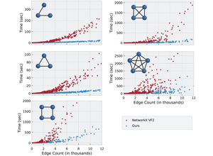
Not, so far, a competitive advantage in mainstream deep learning. The
architectures that dominate practice were not derived from neuroanatomy.
The reverse direction, which is currently stronger
Machine learning has contributed far more to connectomics than the reverse: dense
segmentation, synapse detection, error detection, and automated proofreading candidate
generation are all learned systems, and none of the petascale datasets would exist
without them. When you write about NeuroAI, note the asymmetry. It is the accurate
description of the present state and it costs nothing to be right about.
Visual training set
These are concept and tooling slides from the source decks, several of them historical — use them for the framing rather than the numbers. For each panel, ask what null model its implied claim would need, since §2 shows the same data yielding “2.9-fold enrichment” or “no detectable effect” depending on a choice made before any test is run.
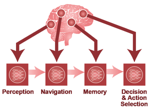
Techtalk S10: The motivating question linking natural and artificial intelligence. Hold it against the asymmetry in §5: machine learning has given connectomics far more than the reverse so far, and saying that plainly is part of writing about NeuroAI credibly.
Techtalk S11: Brain data, framed for analysis. Before any statistic, the six construction choices in §1 have to be made — node, edge, weight, direction, inclusion, boundary — and each changes the answer. A graph is a versioned artifact with recorded parameters, not a script someone ran once.
Techtalk S12: The reverse-engineering analogy. Ask what the analogy assumes a wiring diagram supplies: synapse counts are a proxy for strength and not synaptic weights, and sign, short-term dynamics, plasticity state, and neuromodulatory context are all absent.
Techtalk S13: A NeuroAI pipeline. The strongest result type it can support is a connectome-constrained model — fix connectivity from the measurement, fit what remains, predict responses that are then tested. That is the version where the connectome removes free parameters rather than decorating a figure.
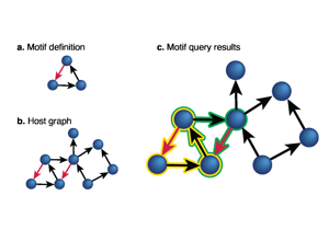
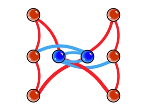
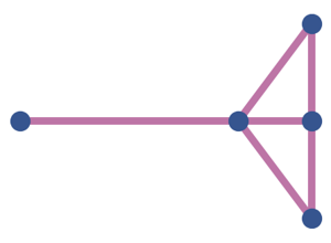
Techtalk S24: Motif search as a concept. A motif is enriched only relative to a null, so ask what would count as the uninteresting explanation here — degree heterogeneity, spatial proximity, or cell-type composition — and require the null to preserve it.
Techtalk S26: The turn from concept to query tooling. Note what a declarative query does not do for you: it returns counts against whatever graph you built, carrying every §1 construction choice, including the synapse threshold that quietly removed most of your edges.
Techtalk S31: Subgraph isomorphism, the computational core. The hard part in practice is statistical rather than algorithmic — triad counts are strongly correlated with one another, so treating the sixteen classes as independent tests overstates confidence and argues for permutation-based inference.
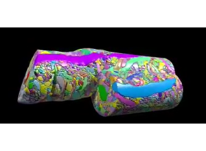
Techtalk S32: A performance benchmark. Read it as historical, per the attribution below, and read benchmarks generally the way the atlas advises — scores on small, clean volumes systematically overstate performance on production data with artifacts, rare morphologies, and volume boundaries.
Techtalk S33: Throughput and scale. Scale changes what is countable, not what is inferable: a larger graph tightens the error bars on a statistic and does nothing about the null-model choice or the merge-error bias that decide whether the statistic means anything.
Techtalk S39: A hypothesis expressed as a scan across the graph. Count the tests, including those you run and do not report — sweeping one hypothesis over many candidates is a multiple-comparison problem, and the correction has to cover the whole sweep.
Techtalk S42: Motif query syntax. Its real value is that the motif definition becomes an explicit, reviewable artifact instead of a description in prose — which is what turns “pre-register the motif and the null” into a practical instruction rather than an aspiration.
Techtalk S44: Motif comparison across development. Comparisons are the most durable result type in this field because a shared reconstruction bias partly cancels between the two sides — the same reasoning behind preferring within-dataset comparisons in Unit 06 §4.
Module13 L3 S03: Project overview. Work backwards from whatever the endpoint claim is, because inclusion criteria — which cells enter the graph at all — is the highest-leverage and least-reported decision in §1.
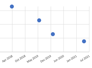
Module13 L3 S11: Data growth. In a connectome dataset growth usually means proofreading continued, so a re-run against a later materialization giving different numbers is correct behavior rather than a bug — provided the version is stated (Unit 04 §2).
Module13 L3 S14: A processing comparison. Ask what is held constant across the arms being compared; if the graphs came from different construction parameters or different materialization versions, the comparison is measuring the pipeline rather than the biology.
Module13 L3 S20: Connectivity estimation. Estimation inherits reconstruction error asymmetrically — merges inflate dense motifs superlinearly while splits deflate everything roughly proportionally — so the residual bias points toward the more interesting answer rather than away from it.
Module13 L3 S24: A classification model built on connectivity. Where connectivity-derived clusters agree with morphological or transcriptomic types you have converging evidence for a type; where they disagree, that disagreement is the finding, and it should not be resolved by quietly picking the preferred answer.
Module13 L3 S29: Late-stage synthesis. This is where the error-sensitivity check belongs: perturb the graph at your own measured merge and split rates, recompute the statistic across many perturbations, and report the spread as an error band before a reviewer finds it for you.
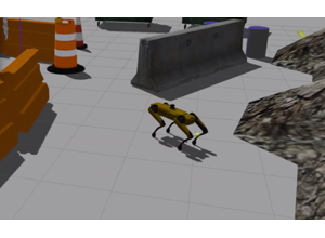
Module13 L3 S37: The application stage. Scope the claim explicitly — a connectome constrains the space of possible dynamics, and it is not weights, not dynamics, and not a runnable brain. Stating that plainly costs nothing and is what makes the rest credible.
Attribution: NeuroAI and outreach source decks from the extraction package. Historical figures (including 2021 techtalk materials) are used for technical context; interpret benchmark claims as historical unless independently revalidated.
Lab: a defensible motif analysis (2 hours)
Using a public connectome:
Build the graph. Record every §1 decision explicitly in a config dict at the
top of your notebook, including the materialization version.
Describe it. Node count, edge count, density, in- and out-degree distributions
(plot on log axes), synapses-per-connection distribution.
Count triads. Use networkx.triadic_census or an equivalent.
Build three nulls: Erdős–Rényi, degree-preserving (double-edge-swap rewiring,
≥ 1,000 samples), and — if soma positions are available — distance-preserving.
Compare. For each triad class, report observed, null mean, null sd, z, and the
corrected p-value. Say how many tests you ran.
Sensitivity. Re-run steps 1–5 at a second synapse threshold. Report what changed.
Error simulation. With a stated merge/split rate, perturb the graph 100 times,
recompute your headline statistic, and report the error band.
Write the result in three sentences: what you found, under which null, with
which caveats. Then write the sentence you are not claiming (Unit 01, step 7).
Rubric
Not yet
Proficient
Strong
Construction
Undocumented
All six decisions recorded, version pinned
Sensitivity to the threshold decision measured and reported
Null choice
ER only
Degree-preserving used
Multiple nulls compared; the “uninteresting explanation” written out in words
Multiple comparisons
Ignored
Corrected
Corrected, count of tests reported, permutation-based inference used to respect dependence
Error sensitivity
Absent
Discussed
Simulated with measured rates; error band reported on the effect size
Interpretation
Effect size stated as fact
Caveats present
Bin A/B/C discipline; explicit non-claim; result stated under each null
Reproducibility
Notebook only
Version and parameters recorded
Another person could re-run it and get the same numbers
If your result vanishes under the degree-preserving null
That is a result, and reporting it is more valuable than most positive findings in
this area.
Concretely, “reciprocity in this circuit is fully explained by degree distribution
and spatial proximity” tells the field something durable and hard to obtain: it
constrains the space of wiring rules that need explaining. Papers reporting motif
enrichment against weak nulls have already been published and will need revisiting;
a clean negative result against a strong null does not.
Write it up. Report all three nulls in a table. State the effect size under each.
Do not go looking for a fourth null that restores significance — and if you do try
other nulls, report every one you tried, because “we tested until it worked” is a
multiple-comparison problem that no correction can repair after the fact.
Common errors and how to recover
Erdős–Rényi as the default null. Recover: use degree-preserving as your minimum
null in a connectome, and add distance whenever soma positions exist.
Unreported synapse threshold. Recover: state it, and report the headline result at
two thresholds.
Ignoring merge-error bias. Recover: run the error simulation in §3 and put the
band in the figure.
Treating triad tests as independent. Recover: permutation inference; report the
number of tests.
Overclaiming NeuroAI relevance. Recover: describe what the connectome constrained
in a specific model, not what it might inspire in general.
Analysis against an unpinned segmentation. Recover: pin the materialization
version (Unit 04 §2). Put it in the figure caption.
The norm behind this unit
Some of what this unit teaches is technique. Some of it is professional norm — the
things experienced people do without being asked, and which nobody states out loud
because they assume you already know. Those are worth naming, because they are
distributed unequally by background rather
than by ability.
From this unit:
Report how many tests you ran — including the ones you ran and did not report.
This is the norm that separates an analysis from a fishing expedition, and it is almost never taught directly.
Report the effect under every null model you tried, not the one that worked.
If you went looking for a fourth null after three failed, that is a multiple-comparison problem no correction can repair afterwards. Say what you tried.
Write the sentence describing what would make the result uninteresting, before choosing a null.
If you cannot write it, you do not yet know what you are testing.
The collected set, and why making these explicit is a fairness intervention rather than
etiquette, is in the hidden curriculum.
What this unit does not cover
Biophysical modeling, detailed statistical theory for random graphs, and functional
data analysis. It also does not cover comparison across imaging modalities — see
Unit 02 for why cross-modality comparison of connectivity claims is delicate.
Keep at hand:Atlas and Connectomics Reference — not a tenth unit but the lookup table for every dataset figure this unit cites; the track itself ends here
Instructor and reference notes
Evidence pack: papers and datasets
This unit is anchored to canonical papers and datasets used in connectomics practice. Use these as required preparation before activities.
Define a motif/null-model analysis pair and interpret uncertainty.
Separate exploratory from confirmatory claims in reports.
Capability development brief
Capability target: Build defensible connectome analysis workflows with robust statistical controls and reproducible inference.
Required expertise
Network neuroscientist (graph and motif interpretation)
ML scientist (representation learning and model validation)
Statistician (null models, uncertainty, and multiple testing)
Core concepts to teach
Motif inference: Testing whether local wiring motifs exceed chance under appropriate null models.
Representation validity: Verifying that learned embeddings preserve biologically meaningful structure.
Inference discipline: Separating exploratory findings from confirmatory claims.
Capability exercise
Motif-to-Model Pipeline Lab - Run a complete analysis from graph extraction to interpretable statistical output. The lab above is the graded version of this exercise; do that one.
Assessment artifacts
Analysis plan with preregistered tests and null models.
Reproducible notebook/report package with provenance metadata.
Related concepts
Motif Analysis and NeuroAI
Build query-driven motif workflows with statistical controls and reproducible execution.