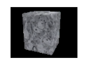
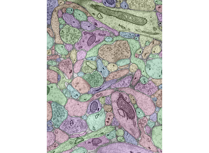
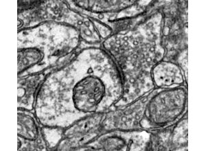
How automated segmentation fails, which metrics reveal which failure, and how to run proofreading as a prioritized, measured, budget-bounded operation rather than an open-ended cleanup.
Key community resources for this unit:
FlyWire / Codex
— Dorkenwald et al. (2022), "FlyWire: online community for whole-brain connectomics," Nature Methods 19:119–128 Leading real-world example of AI-assisted segmentation plus community/crowd-sourced proofreading of a whole-brain EM connectome (Drosophila).
Dorkenwald et al. (2024)
— "Neuronal wiring diagram of an adult brain," Nature 634:124–138 The completed FlyWire connectome paper — a capstone reference showing proofreading-at-scale outcomes.
CAVE
— Dorkenwald et al. (2025), Nature Methods 22:1112–1120 Its core function is proofreading and annotation versioning at scale (see Unit 04).
Before you start
Time
Self-study ~4.5 h: about 2.5 h of reading plus the 2 h lab. Taught: a 95 min session, per the lecture plan. Deck: the unit’s slide deck is scoped to 60 min and does not follow the plan slide for slide.
Prerequisites
Units 03–07. Unit 06’s error-cost reasoning is used heavily here.
You need
A proofreading-capable viewer (Neuroglancer against a CAVE dataset, or webKnossos) and an account
You finish with
A proofreading plan with an explicit stopping rule, a triage ranking, and a defended budget
The framing that makes this unit different from a tool tutorial. Proofreading is
not “fixing the segmentation until it is right”. Segmentation is never right, and at
petascale nobody will ever look at most of it. Proofreading is an allocation problem
under a fixed budget: which corrections, in which order, stopping when.
Teams that treat it as cleanup run out of money with a half-corrected volume and no
defensible claim. Teams that treat it as allocation deliver a specific scientific
result with quantified error bounds. The difference is entirely in how the work is
prioritized and when it is declared finished.
[!TIP]
Looking for Hands-On Tracing Walkthroughs & Tool Tutorials?
Check out the EM Proofreading Tutorials & Community Practice Guide for step-by-step Neuroglancer/CAVE keybinding cheat sheets, false merge/split visual diagnosis, synapse validation criteria, and direct links to the FlyWire Academy and EyeWire platforms.
What you’ll be able to do
Name the error types automated segmentation produces and rank them by cost for a given endpoint.
Choose the right metric for a given question and say what each metric hides.
Build a triage ranking that prioritizes by effect on the endpoint rather than by conspicuousness.
Define a stopping rule that is checkable by someone other than you.
Estimate proofreading effort and defend the estimate.
1. How automated segmentation works, briefly
Enough to reason about its failures. (Full detail: Unit 04 §1 and the content library.)
For a worked case of everything in this unit on one real dataset, see
H01, Step by Step:
it shows flood-filling network output overlaid on raw EM, why H01 ships two
agglomerations that trade merge errors against split errors in opposite directions, the
measured split/merge correction counts for each, and what 104 proofread cells out of
16,087 neurons means in practice.
The affinity/agglomeration family. A network predicts, per voxel, the affinity
between neighboring voxels. Watershed at a conservative threshold produces
supervoxels that are deliberately too small. An agglomeration step then merges
supervoxels into objects, using mean affinity, learned agglomeration, or shape-based
descriptors that let the model reason about whether a merge produces a plausible
neurite shape.
The flood-filling family. A network iteratively grows one object from a seed,
maintaining a mask and repeatedly asking “does this next voxel belong?” This produces
strong results because the network sees the object it is building, but it is
sequential and expensive.
Where both fail, structurally:
Thin processes. A 60 nm spine neck at 40 nm z-resolution may appear in only one
or two sections. There is very little evidence to work with, so spine necks are a
perennial source of splits.
Steep z-trajectories. Anisotropy again. A process crossing sections at a shallow
angle to the imaging plane presents a small, rapidly-moving cross-section.
Membrane contact. Two membranes tightly apposed over many sections may not be
separable, especially with weak staining (Unit 03).
Artifact regions. Folds, charging, missing sections — the network was not
trained on tissue that does not exist.
Rare morphologies. Anything under-represented in the training set: unusual cell
types, developmental stages, pathology, and — importantly — the boundaries of the
volume.
The design choice that shapes everything downstream: the pipeline is deliberately
tuned to over-segment. It prefers splits to merges. That is a decision about which
error is cheaper to repair, and it dictates that proofreading is mostly joining.
2. Error taxonomy and cost
Error
What it is
Detection difficulty
Cost
Who finds it
Split
One neuron in multiple pieces
Easy — arbor looks truncated
Bounded, local, visible
Automated heuristics (endpoint detection) and humans
Merge
Two neurons fused
Hard — object looks fine unless you check morphology
High — manufactures local false connectivity (Unit 07 §1)
Humans
Orphan fragment
A piece belonging to no traced object
Easy to count
Low individually; large in aggregate as unattributed volume
Automated
False synapse
Detection where no synapse exists
Medium
Inflates degree; worst on weak (1-synapse) connections
Human verification on a sample
Missed synapse
Real synapse not detected
Hard (you are looking for absence)
Deflates degree, non-uniformly by synapse size
Human verification on a sample
Wrong synapse partner
Correct cleft, wrong pre- or post- assignment
Hard
Direction/identity error, as in Unit 06
Human
The asymmetry, stated once more
Splits are visible and bounded. Merges are invisible and unbounded. A split leaves
evidence of itself — a neuron that stops in mid-neuropil. A merge leaves an object
that looks like a neuron and is not. The whole architecture of the field, from
watershed thresholds to proofreading protocols to quality metrics, is organized around
this asymmetry.
Check yourself
On your 50-cell analysis set, the endpoint detector lists 300 split candidates
and the morphology-implausibility detector lists none. A colleague concludes the set is
effectively merge-free and proposes spending the whole budget on splits. What is wrong
with the inference?
An empty merge queue measures the detector, not the segmentation.
The two queues are not symmetric. A split announces itself — a neurite that stops in
mid-neuropil without tapering — so an endpoint detector finds most of them. A merge
does not: the implausibility detector only fires on the merges that produce something
biologically impossible, such as two somata in one object, or ribosomes and
presynaptic vesicle clusters in the same process. A merge between two plausible
neurites looks like an ordinary neuron and passes straight through. So “no merge
candidates” is consistent with no merges, and equally consistent with merges of the
kind the detector cannot see — which are the expensive kind.
The table also tells you why the split queue is long: the pipeline is deliberately
tuned to over-segment. Three hundred splits is the design working, not evidence that
merges are rare.
What settles it is the §3 procedure: exhaustively proofread a random sample of the 50
cells, to a standard above production, and see whether any merges turn up and how far
fixing them moves the endpoint. Then allocate the budget — and remember that merges
outrank splits at equal size.
Generalizable principle: absence from a queue is only evidence of absence for errors
the detector can see. Know which errors your detectors are blind to before you read an
empty list as a clean bill.
3. Metrics: what each one is blind to
The content library has the mathematics; this section is about choosing.
Metric
Measures
Blind to
Use when
Variation of Information (VI)
Total disagreement between two segmentations, decomposable into split and merge components
Object size — a merge of two tiny fragments and a merge of two full neurons contribute very differently, and not in the way you might want
Comparing segmentation versions on the same volume
Expected Run Length (ERL)
Mean error-free path length along skeletons
Merges, unless explicitly penalized; also insensitive to small dangling fragments
Tracing-oriented questions: “how far can I follow a neurite before hitting an error?”
Edge precision / recall
Correctness of connections in the derived graph
Weights all edges equally, so a 1-synapse and a 50-synapse connection count the same
Graph-level claims
Synapse precision / recall
Correctness of detected synapses
Assumes correct segmentation underneath — a synapse assigned to a merged object scores as correct
Synapse-level claims
Completeness (per neuron)
Fraction of a neuron actually reconstructed
Says nothing about correctness of what is there
Per-cell claims like input counts
Use at least two metrics from different rows, and always report VI’s split and
merge components separately. A single VI number can improve while merges get worse,
because the split component dominates. That is a real and common way to ship a
regression.
The metric that actually matters
None of the above. The metric that matters is the effect on your endpoint.
Concretely: if your result is “cell type A makes 3× more synapses onto type B than
onto type C”, then the question is not “what is our VI?” It is: how much would the
observed 3× change under a plausible correction of the remaining errors?
Procedure:
Take a random sample of the cells in the analysis — 20 is often enough to be
informative.
Proofread them exhaustively, to a standard well above your production standard.
Recompute the endpoint on that sample, before and after.
Report the shift. “Exhaustive proofreading of a 20-cell sample changed the ratio
from 3.1 to 2.8” is a far stronger statement about data quality than any VI value,
and reviewers understand it immediately.
This costs a few dozen person-hours and it converts “we proofread the data” into a
quantified error bound. It is the single highest-value practice in this unit.
Check yourself
Version B of your segmentation has lower total VI than version A, and your
team wants to ship it. What do you check first?
Decompose VI into split and merge components.
Total VI is dominated by whichever component is larger, and in an over-segmented
pipeline that is usually splits. Version B may have reduced splits (perhaps by more
aggressive agglomeration) while increasing merges — and the total would still
improve.
Since merges are the expensive error, a “better” total VI with worse merges is a
regression for connectomics purposes, even though the headline number improved.
Also check: ERL (does tracing actually get easier?), and — decisively — recompute
the endpoint metric on a fixed evaluation set of neurons. Ship on the endpoint, not
on the aggregate score.
4. The production proofreading loop
1. SEED       Select target cells by scientific priority, not by convenience
                or by which segment happens to be biggest.
2. TRIAGE     Rank candidate corrections by expected effect on the endpoint.
3. CORRECT    Apply merges/splits with evidence recorded (Unit 05 evidence chains).
4. VERIFY     Independent second pass on a sample; measure agreement.
5. MEASURE    Recompute quality metrics AND the endpoint metric.
6. STOP       Apply the stopping rule. Record the state as a release.
Triage: ranking corrections
Rank by expected change in the endpoint per unit of annotator time, not by error
conspicuousness. In practice this means scoring candidates on:
Proximity to the endpoint. An error on a cell in your analysis set outranks an
identical error on a cell that is not.
Error type. Merges outrank splits at equal size, because merges corrupt rather
than truncate.
Size. A split that truncates 60% of an arbor outranks one that loses a 3 µm
twig — but note that a small merge can be worse than a large split, so size
ranks within type, not across types.
Path centrality. An error on the primary neurite near the soma disconnects
everything distal to it. Errors near the root are worth far more than errors at the
tips.
Cost to fix. A correction requiring 40 minutes of careful tracing through a fold
may lose to five 5-minute corrections elsewhere.
Automated candidate generation feeds this queue: endpoint detectors (a neurite
that stops without tapering to a natural ending is a split candidate), morphology
implausibility detectors (an object with two somata; an object with both ribosomes and
presynaptic vesicle clusters — the Unit 06 alarm), and agglomeration-confidence
thresholds. Humans then adjudicate a ranked queue rather than browsing.
Worked example: three candidates, one annotator-hour
Setup: the study needs 200 proofread layer 2/3 pyramidal cells for a
cell-type targeting endpoint — fraction of input synapses by presynaptic class,
per cell. The queue’s top three candidates, with one annotator-hour available
before today’s verification pass:
A — a split: an analysis-set cell’s primary apical dendrite truncated
close to the soma, detaching roughly 60% of the arbor. Estimated fix: 10 min.
B — a glia–neuron merge: a fine astrocytic process fused onto another
analysis-set cell’s basal dendrite. Estimated fix: 20 min — thin, and it
needs care.
C — a conspicuous merge: two somata in one object, flagged by the
morphology detector. Neither cell is in the analysis set. Estimated fix: 15 min.
Score them on the five factors, with the assumptions said out loud.
Proximity to the endpoint. A and B sit on analysis-set cells. C looks
dismissible — but not yet: C could still corrupt the endpoint indirectly, if
either fused neuron is presynaptic to an analysis cell, because the merge
scrambles the presynaptic identity of those inputs. Check the partner lists —
two minutes — and find no synapses onto the 200. Only now does C actually drop.
The assumption “C does not touch the endpoint” has been tested, not presumed.
Error type. B corrupts: the astrocytic path drags past synapses the dendrite
never contacted, and those false inputs enter the class fractions silently
(Unit 07 §1). A truncates: the input count is undercounted, but visibly — the
cell fails the “dendrite complete” criterion for its level and is excluded until
fixed. An unfixed A delays a cell; an unfixed B poisons one.
Size and path centrality. Within splits, A is severe — near the root, with
most of the arbor detached. But size ranks within type, not across types: A’s
60% does not outrank B’s merge.
Cost to fix. A is half B’s price. Per expected endpoint change per minute, B
still wins: removing silent corruption beats accelerating a visible, bounded
repair.
The hour: B (20) + A (10) + the partner check on C (2) = 32 minutes. The
remaining 28 do not go to C — its only argument was conspicuousness, which is
not a factor — but to the next analysis-set candidates in the queue: roughly
five more corrections at a five-minute median. C is logged with a reason,
unfixed.
Transferable principle: rank by expected endpoint change per annotator
minute, and test the “obviously irrelevant” candidate before dismissing it —
two minutes of checking is part of the triage, not overhead. This is the
exercise Part B of the lab asks you to write down for your own candidates, with
the weights stated in advance.
Stopping rules
This is where most projects fail, because “keep going until it looks good” has no
termination condition and no defensible reporting.
A stopping rule must be stated in advance, measurable, and tied to the
endpoint. Examples of usable rules:
Convergence: “Stop when a second independent proofreading pass over a 20-cell
sample changes the endpoint metric by less than 5%.” This is the strongest general
rule — it directly measures whether more effort would change the answer.
Budget with declared coverage: “Proofread to level N on 200 cells; report per-cell
proofreading level with every result; make no claims about cells below level N.”
Threshold: “Every cell in the analysis set has ≥ 95% of its dendritic arbor
recovered relative to a manually traced reference on a validation subset.”
Levels are the practical mechanism. Rather than a binary proofread/not-proofread,
define levels — e.g. L0 raw, L1 gross merges removed, L2 dendrite complete,
L3 axon extended, L4 exhaustive — with written criteria for each. Then:
Cells carry their level as metadata.
Analyses state the required level and exclude cells below it.
Effort is directed at raising specific cells to a specific level, which is a
plannable task with an estimable cost.
The reporting rule. Every connectomics result should state the proofreading
level of the cells it rests on, and the criteria defining that level. A result that
does not is uninterpretable, because the reader cannot tell whether a low measured
connection count reflects biology or incompleteness.
Check yourself
A draft methods section says: "All 200 cells were proofread." A reviewer calls it
uninterpretable. What does the sentence need to become?
It needs a level, the criteria for that level, and the rule that decided when to
stop. “Proofread” on its own covers everything from gross merges removed to
exhaustive, and a reader cannot tell which — so a low connection count could be
biology or incompleteness.
A version that survives review states:
The level and its written criteria — for example, “all 200 cells were proofread
to L2, dendrite complete, defined as…”, with the definition given or cited.
Per-cell metadata — every cell carries its level, and cells below the level the
analysis requires are excluded, with the number excluded reported.
The stopping rule, stated in advance — for example, the convergence rule: a
second independent pass over a 20-cell sample changed the endpoint by less than 5%.
The measured shift — what exhaustive proofreading of a sample did to the
endpoint, the §3 number that turns “we proofread” into an error bound.
The first sentence is the one the reviewer objected to. The fourth is the one that
answers the question the reviewer was really asking: would more proofreading have
changed the result?
Generalizable principle: a data-quality claim is interpretable only when a reader
can say what would count as it being false. “Proofread” cannot fail; “L2 by these
criteria, stopped by this rule, endpoint shift of this size” can.
5. Human factors, because this is a labor operation
At petascale, proofreading is a workforce, and it behaves like one.
Training and calibration. New annotators need a calibration set with known
answers, and periodic recalibration — drift is real and it is gradual. Run the Unit 05
consensus round and the Unit 06 calibration lab as onboarding, then repeat quarterly.
Measure agreement, not just throughput. Throughput alone rewards speed over
correctness, and it will get you exactly that. Track: inter-annotator agreement on a
shared subset, and per-annotator error rate on gold-standard tasks seeded invisibly
into the normal queue. Discuss agreement openly; treat disagreement as protocol
feedback rather than individual failure.
Fatigue is a data-quality variable. Error rates rise across a long session.
Structure work in bounded blocks and rotate task types.
Community proofreading works, with structure. The FlyWire whole-brain connectome
was completed with millions of edits from a large distributed community over several
years — an existence proof that this scales beyond a single lab. What made it work was
not enthusiasm but infrastructure: task queues, automated candidate generation, tiered
permissions, edit provenance, expert adjudication for hard cases, and clear
attribution.
The tooling requirement that follows. Every edit records who, when, what, and
ideally why. This is not surveillance; it is what lets you (a) roll back a bad batch,
(b) identify a training gap when one annotator’s edits are systematically different,
and (c) reconstruct the state of an analysis at any past time (Unit 04 §2).
Visual training set
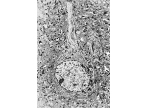
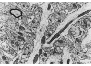
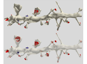
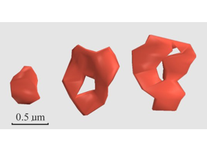
The first six panels carry ultrastructure cues forward from Units 05–06; the rest are pipeline context. Use them as triage practice rather than identification practice: for each one, ask what error a wrong reading would produce, and whether that error is a bounded, visible split or an unbounded, invisible merge.
RIV-ULTRA S06: Orientation for proofreading judgment. Set the frame before touching anything: proofreading is allocation under a fixed budget rather than cleanup, so the question about any candidate correction is what it changes about the endpoint per minute of annotator time.
RIV-ULTRA S09: Synapse features that drive correction decisions. Apply the Unit 05 criteria before crediting a detection — a synapse assigned to a merged object still scores as correct under synapse precision, which is exactly what that metric is blind to.
RIV-ULTRA S11: Vesicle and organelle cues on ambiguous objects. Look for combinations that cannot coexist in one cortical process; implausible-morphology detection is how merges get found at all, since a merged object otherwise looks like a perfectly ordinary neuron.
RIV-AXDEN S13: Axon against dendrite, for identity checks. Every edge direction in the final graph rests on this call, and a reversed edge is not noise — it deletes a true edge and adds its opposite. Audit the edges whose direction would change your conclusion rather than auditing uniformly.
RIV-AXDEN S18: An edge case at high risk of a wrong correction. Estimate cost to fix before committing: a forty-minute trace through a difficult region loses to five five-minute corrections elsewhere, unless the cell is in your analysis set and the error sits near the root of the arbor.
RIV-ULTRA S17: A dendrite (D) with two spines (s1, s2), each opposite a vesicle-filled bouton. §1 names thin spine necks as a perennial source of splits. If a neck is lost, the spine head becomes a separate fragment and its synapse leaves the dendrite's input count without anything looking wrong at the dendrite — which is why orphan fragments, cheap one at a time in the §2 table, add up.
Module14 L2 S03: A method overview with QC in the loop. Ask where the measurement points are: a pipeline without a fixed evaluation set of neurons can only report aggregate scores, and aggregate scores are how a merge regression ships behind an improved total VI.
Module14 L2 S08: The transition from voxels to graph. Everything upstream of this point is repairable; everything downstream inherits whatever came through. Note that edge precision and recall weight a one-synapse and a fifty-synapse connection equally, which hides the connections most vulnerable to error.
Module14 L2 S09: Automated detection feeding human work. The right reading is candidate generation rather than automation: detectors propose a ranked queue — endpoint detectors for splits, implausibility detectors for merges — and humans adjudicate the ranking instead of browsing the volume.
Module14 L2 S10: A quality-relevant processing stage. For whatever this stage emits, ask what provenance travels with it — who, when, what, and ideally why — because rolling back a bad batch and detecting one annotator’s drift both depend on that record existing.
Module14 L2 S13: Evaluation and metrics reporting. Hold it to the rule in §3: at least two metrics from different rows, VI always split into its merge and split components, and the number that actually decides anything is the shift in your endpoint after exhaustively proofreading a twenty-cell sample.
Attribution: Pat Rivlin training materials for RIV-* visuals; outreach visuals from module14 lesson2 extraction. Some planned IDs were unavailable in extracted thumbnails and were replaced with nearest available alternatives.
Lab: proofreading plan with a defended budget (2 hours)
Part A — hands on (60 min).
In a proofreading-capable viewer on a public dataset:
Pick a neuron with visible errors. Trace its arbor and log every error you find:
type, location, estimated size of the affected arbor fraction, and estimated fix
time.
Fix the three highest-impact errors by your own ranking, and record your ranking
rationale before fixing.
After fixing, recount the neuron’s input synapses. Report the change from before.
This number is your personal demonstration of why proofreading level must be
reported with results.
Note one error you chose not to fix, and why.
Part B — the plan (60 min).
Your project needs 200 proofread layer-2/3 pyramidal cells to test a cell-type
targeting hypothesis. Write a two-page proofreading plan:
Endpoint metric, stated precisely, with units.
Proofreading levels, defined with written criteria a new annotator could apply.
State which level each part of your analysis requires and why.
Triage ranking rule, with the factors from §4 and their relative weights. Give
a worked example applying it to two competing candidate corrections.
Stopping rule, stated so that a person who is not you could determine whether it
has been met.
Budget: person-hours, derived from your own Part A timing extrapolated with
stated assumptions. Show the arithmetic.
Quality plan: which metrics, on what sample, at what frequency; how you will
measure inter-annotator agreement; and the endpoint-shift measurement from §3.
What you will report in the eventual paper about data quality — write the
actual methods paragraph.
Rubric
Not yet
Proficient
Strong
Endpoint
Vague
Precise with units
Precise, and the required proofreading level is derived from it rather than asserted
Levels
Binary done/not-done
Levels defined
Criteria are operational — two annotators would assign the same level
Triage
“Fix the big ones”
Multi-factor ranking
Weights justified, worked example given, cost-to-fix included
Stopping rule
Absent or unfalsifiable
Stated and measurable
Convergence-based, tied to the endpoint, checkable by a third party
Budget
Guessed
Derived from measured timing
Assumptions stated, sensitivity considered, and a contingency for the hard tail
Quality plan
Metrics named
Metrics with sampling plan
Includes endpoint-shift measurement and inter-annotator agreement
Reporting
Not attempted
Mentions proofreading
A methods paragraph a reviewer would accept, with per-cell level reported
The estimation trap in step 5 — read after drafting your budget
Almost everyone underestimates, and almost always the same way: by extrapolating
from the median neuron.
Proofreading time per neuron is heavy-tailed. Most cells are quick; a minority
consume many times the median because they sit in an artifact region, have an
unusually extensive axon, or are tangled with a neighbor across many sections. If
you budget median × 200, you will be short — and the shortfall will land at the end
of the project, when it is most damaging.
Better practice:
Estimate from the mean, and estimate the mean from a sample large enough to
include tail cases (in practice, don’t trust a sample of fewer than ~10–15 cells).
Or: budget median × N, and add an explicit contingency for the tail, stated as a
separate line item.
Or best: define your stopping rule so that pathological cells are excluded by
policy after a stated time cap, and report the exclusion rate. A stated 6%
exclusion rate is honest and cheap; an unbudgeted tail is neither.
This is also a good illustration of why the stopping rule and the budget must be
designed together rather than sequentially.
Common errors and how to recover
Proofreading without a stopping rule. Recover: write one now, tie it to the
endpoint, and get someone else to confirm they could evaluate it.
Optimizing the aggregate metric. Recover: fix an evaluation set of neurons and an
endpoint metric; ship on those.
Triage by conspicuousness. Recover: score candidates on a written rubric; audit a
sample of decisions against it.
Unreported proofreading level. Recover: attach level metadata per cell; filter
analyses by level; state it in the methods.
Rewarding throughput alone. Recover: publish agreement statistics alongside
throughput and discuss them as protocol feedback.
Assuming the error rate is uniform. It is not — it is much higher near volume
boundaries, in artifact regions, and for thin processes. Recover: report error rate
by region and by process caliber, and let that drive both triage and the caveats.
The norm behind this unit
Some of what this unit teaches is technique. Some of it is professional norm — the
things experienced people do without being asked, and which nobody states out loud
because they assume you already know. Those are worth naming, because they are
distributed unequally by background rather
than by ability.
From this unit:
State the proofreading level of the cells a result rests on.
Without it a reader cannot tell whether a low connection count is biology or incompleteness. Almost no published analysis includes this, which is exactly why including it is noticed.
Define the stopping rule before you start, and make it checkable by someone else.
“Until it looks good” is not a stopping rule. Writing one down in advance is what converts proofreading from open-ended cleanup into a plannable task.
Report what you excluded and why.
A stated 6% exclusion rate is honest and cheap. An unbudgeted tail discovered at the end is neither.
The collected set, and why making these explicit is a fairness intervention rather than
etiquette, is in the hidden curriculum.
What this unit does not cover
Segmentation model architecture and training in depth, and the statistical analysis of
the resulting graph (Unit 09). Tool-specific keyboard workflows change too fast to
document here; use the vendor documentation and record your team’s conventions in your
own protocol.
Prioritize proofreading corrections by biological impact.
Report QC metrics tied to release/no-release decisions.
Capability development brief
Capability target: Run a production-ready proofreading workflow that prioritizes corrections by scientific impact.
Required expertise
Segmentation scientist (model behavior and failure modes)
Proofreading operations lead (queueing and throughput strategy)
Quantitative QC analyst (precision/recall and uncertainty metrics)
Core concepts to teach
Merge/split taxonomy: Standardized categorization of topological reconstruction errors.
Impact-weighted triage: Prioritizing corrections that most affect downstream biological conclusions.
Quality reporting: Translating correction activity into interpretable, reproducible QC metrics.
Capability exercise
Proofreading Queue Optimization - Balance correction quality and throughput under limited expert time. The lab above is the graded version of this exercise; do that one.
Assessment artifacts
Proofreading SOP with triage rules and escalation criteria.
QC dashboard definition with required metrics and update cadence.
Related concepts
Proofreading and QC
Classify error modes, apply correction workflows, and tie decisions to quantitative quality metrics.