The tissue-to-image-stack chain in practical detail: fixation and staining chemistry, sectioning, imaging parameters, and an artifact catalog mapped to downstream reconstruction cost.
Want to see this in real data?EM figure library collects every micrograph on this site, and H01, Step by Step carries real electron micrographs of human cortex — rendered straight from the public H01 volume — from whole-sample down to individual synapses, alongside the pipeline that produced them.
This page itself is still text-only on the diagram side. For equipment schematics and further depth, see:
Peters, Palay & Webster, The Fine Structure of the Nervous System (3rd ed.) — the standard reference for identifying ultrastructure in EM images
MICrONS Explorer — real acquisition photos, diagrams, and dataset specs
Before you start
Time
Self-study ~3.5 h: about 2 h of reading plus the 90 min lab. Taught: a 90 min session, per the lecture plan. Deck: the unit’s slide deck is scoped to 60 min and does not follow the plan slide for slide.
Prerequisites
Units 01–02
You need
Access to any public EM volume in Neuroglancer (MICrONS, FlyWire, or H01 all work)
You finish with
A completed acquisition QA report on a real volume, with artifacts localized and costed
The governing fact of this unit: acquisition quality sets a ceiling on
reconstruction quality that no amount of downstream machine learning or proofreading
labor can raise. A fold destroys the tissue. A missing section destroys the
continuity. You can annotate around damage, but you cannot recover what was never
imaged. This is why acquisition QA is not a formality — it is the highest-leverage QC
in the entire pipeline, and it is the one most often deferred.
What you’ll be able to do
Explain what each major step of the sample-prep chain contributes, and what
specific image defect appears when it fails.
Read an EM image and name the likely acquisition cause of a visible defect.
Distinguish artifacts that cost proofreading hours from artifacts that cost
data, and prioritize accordingly.
Compute an acquisition time estimate from pixel rate, volume, and voxel size.
Write an acquisition QA report that a reconstruction team can act on.
1. The preparation chain, step by step
Every step exists to solve a specific problem, and each one introduces a
characteristic failure. Learn the pairs.
1.1 Fixation
What it does. Cross-links proteins to arrest ultrastructure within seconds, before
autolysis and osmotic swelling destroy the extracellular space and the fine processes.
Typical protocol. Transcardial perfusion in rodents with a buffered aldehyde mix —
commonly around 2–2.5% glutaraldehyde plus 2% paraformaldehyde in 0.1 M cacodylate or
phosphate buffer, at physiological pH, often with added calcium. Glutaraldehyde is the
workhorse because it is bifunctional and cross-links rapidly; paraformaldehyde
penetrates faster and buys time.
What failure looks like in the final image.
Swollen astrocytic processes and enlarged extracellular space — the classic
signature of slow or delayed fixation. Neuropil looks “loose”; there are visible
gaps between processes that should be tightly apposite. Downstream cost: actually
makes automated segmentation somewhat easier (more space between objects) but
distorts every geometric measurement, and it means the tissue you reconstructed is
not the tissue that existed in vivo.
Dark, shrunken, hypercontracted neurons — perfusion pressure or osmolarity
problems.
Blood cells retained in vessels — incomplete perfusion; the tissue near those
vessels is likely under-fixed.
Teaching point for annotators. When you see a region of unusually open neuropil,
do not treat it as a segmentation opportunity. Flag it. It is a region where your
geometric measurements — spine neck diameter, apposition area, extracellular
fraction — are not comparable to the rest of the volume.
1.2 Contrast generation (staining)
Biological tissue is nearly transparent to electrons. Contrast comes entirely from
heavy metals bound to specific structures. Membranes are what matters for
connectomics, so the protocol is optimized for lipid.
The standard sequence:
Osmium tetroxide (OsO₄) — binds unsaturated lipids, so it stains membranes. This
is the primary source of the dark membrane outlines you trace.
Reduced osmium (OsO₄ with potassium ferrocyanide) — enhances membrane contrast
and improves staining of internal membranes.
Thiocarbohydrazide (TCH) — a bridging agent. It binds the osmium already in the
tissue and provides new sites for a second osmium exposure. This is the “O-T-O”
amplification step.
Second osmium — deposits more metal onto the TCH bridges.
Uranyl acetate, en bloc — general contrast, particularly nucleic acids and
proteins.
Lead aspartate (Walton’s method) — final contrast enhancement, applied to the
block rather than the section.
The combination is usually called rOTO (reduced osmium – thiocarbohydrazide –
osmium). Two reasons it dominates volume EM: it produces membrane contrast strong
enough to image quickly at low dose, and the metal load makes the block
electrically conductive, which is what makes block-face SEM possible at all
without catastrophic charging.
What failure looks like:
Weak membrane contrast — thin or interrupted membrane outlines. Downstream
cost: the dominant cause of automated merge errors, because the network cannot
find a boundary that is barely there. This is the single most expensive prep failure.
Staining gradient with depth — the block edge is well stained, the center is
pale, because reagents did not penetrate. Common in blocks that are too large.
Downstream cost: segmentation quality varies systematically with position, which
looks like a biological gradient if you are not careful.
Precipitate — small, very dark, irregular particles scattered on the section,
often from lead carbonate formation. Downstream cost: false boundaries and false
synapse detections; usually tolerable at low density.
1.3 Dehydration and embedding
What it does. Water is replaced by solvent (graded ethanol or acetone), then by
epoxy resin (Epon/Araldite, LX-112, Durcupan, Spurr’s), which is polymerized to a
solid block that can be cut at tens of nanometers.
The unavoidable cost: dehydration shrinks tissue, typically on the order of
5–20% linearly depending on protocol. This is systematic, not random. Every absolute
length, area, and volume measurement in EM connectomics is affected. Report
measurements as measured, state the protocol, and prefer ratios and comparisons within
a volume over absolute values compared across studies.
What failure looks like: cracks and tears (usually from too-rapid dehydration or
incompletely infiltrated resin), and resin that is too soft or too brittle to section
cleanly, which shows up at the next step.
1.4 Sectioning or block-face removal
Two families, with different artifact profiles.
Serial sectioning (for ssTEM / ssSEM). An ultramicrotome with a diamond knife cuts
30–50 nm sections, which are collected onto grids, tape (ATUM), or a reinforced
substrate (GridTape). Sections are then imaged, in some cases by many microscopes in
parallel.
Advantage: the block is not consumed by imaging, so a section can be re-imaged at
higher resolution, and imaging can be parallelized across instruments. This is how
petascale volumes get acquired in finite time.
Signature artifacts:lost sections, folds, wrinkles, knife chatter
(periodic bands perpendicular to the cutting direction, from knife or block
vibration), compression along the cutting axis, debris and contamination,
and scratches.
Block-face (SBEM). Image the block face, then shave off a slice with a diamond
knife inside the chamber, repeat. FIB-SEM substitutes an ion beam that mills a few
nanometers at a time, giving isotropic voxels.
Advantage: no section handling means no lost sections and dramatically better
z-alignment. FIB-SEM’s isotropy is the best tracing condition available.
Signature artifacts: the imaged material is destroyed, so nothing can be
re-imaged; charging, since the surface is not conductive-coated between cuts;
and for FIB-SEM, curtaining (vertical striping from uneven milling).
1.5 Imaging
The parameters you will actually be asked about:
Parameter
Typical range
Increase it and…
Decrease it and…
Landing energy (SEM)
1–2 keV
More depth signal, more charging, more beam damage
Better surface specificity, weaker signal
Dwell time per pixel
0.1–2 µs
Better SNR
Faster acquisition, noisier images
Beam current
pA–nA
Better SNR at fixed dwell
Less damage and charging
Tile overlap
5–15%
More robust stitching
Less redundant data, faster
Section thickness (z)
30–50 nm
Fewer sections, faster, cheaper
Better z-continuity, more data
Dose is a budget. SNR improves roughly with the square root of electron dose, and
dose is the product of beam current and dwell time. Doubling SNR costs roughly 4× the
acquisition time. This is why “just image it better” is rarely the answer at petascale
— the honest tradeoff is usually to accept a noisier image and spend the savings on
better segmentation and more proofreading.
Multibeam SEM attacks the throughput term directly: 61 or 91 electron beams
scanning in parallel, aggregating on the order of a gigapixel per second. That is the
technology that moved 1 mm³ from “impossible” to “an eighteen-month project”.
Worked example: acquisition time
A volume is 800 µm × 800 µm × 800 µm at 4 × 4 × 40 nm. Your instrument sustains
0.2 gigapixels per second including overheads. How long?
voxels_xy per section = (800,000 / 4)^2 = 200,000^2 = 4.0 x 10^10 px
sections              =  800,000 / 40   = 20,000
total pixels          = 4.0e10 x 2.0e4  = 8.0 x 10^14 px

time = 8.0e14 / 2.0e8 px/s = 4.0 x 10^6 s ~= 46 days of continuous imaging
Then multiply by your real duty cycle. At 60% uptime this is ~77 days; and this
counts only imaging, not sectioning, not QA, not re-imaging failed sections. When
someone says a 1 mm³ volume takes “about a year”, this is the arithmetic behind it.
Check yourself
Your images show good contrast at the block edges and washed-out membranes in
the center of every section. Which step failed, and what is the fix?
Staining penetration (§1.2). The reagents — most likely osmium, TCH, or lead —
did not reach the block interior. The tell is that the gradient follows block
geometry, not tissue anatomy or acquisition order.
Fixes, in order of practicality: cut smaller blocks (the standard answer — penetration
depth is the constraint, so reduce the distance); extend incubation times;
use microwave-assisted processing; check reagent freshness, particularly TCH.
Diagnostic contrast: if the washed-out region followed acquisition order rather
than block position, you would suspect beam or detector drift instead. If it followed
anatomy (e.g. only white matter), you would suspect a genuine tissue-composition
effect. Always ask which coordinate system the defect lives in — that identifies the
stage that produced it.
2. Artifact catalog with downstream cost
This is the reference table to keep open while doing QA. The right-hand columns are
what turn “the data looks bad” into a decision.
Artifact
How to recognize it
Root cause
Downstream effect
Cost class
Lost section
A z-gap; structures discontinuous across one z index, volume-wide
Section lost during collection
Every process crossing that z must be bridged by inference
Data loss — unrecoverable
Fold
Dark band with duplicated/compressed tissue, usually linear
Section wrinkled on collection
Tissue in the fold is unusable; segmentation splits along it
Data loss in the folded strip
Tear / crack
Sharp-edged gap, often following a vessel
Dehydration or sectioning stress
Local loss; false boundaries at edges
Data loss, localized
Knife chatter
Periodic bands, fixed spacing, perpendicular to cutting direction
Knife or block vibration
Adds false boundaries; raises split rate
Labor — proofreadable
Compression
Section shorter along cutting axis than expected
Knife compresses the section
Systematic geometric distortion; must be corrected in alignment
Labor, plus measurement bias
Charging
Bright streaks or smears trailing the scan direction; local distortion
Non-conductive surface accumulating electrons
Model confidence collapses locally; splits
Labor
Curtaining (FIB-SEM)
Vertical stripes parallel to milling direction
Uneven milling rate
Texture noise; degrades boundary detection
Labor
Weak membrane contrast
Faint or interrupted membrane outlines
Understaining
Merge errors — the expensive kind
Labor, high
Precipitate
Small very dark irregular particles
Staining chemistry
False synapse detections; minor false boundaries
Labor, low
Contamination / debris
Foreign objects, often out of focus
Handling, chamber contamination
Local obstruction
Labor, low
Beam damage
Bubbling, mass loss, progressive contrast change
Excess dose
Degradation that worsens with re-imaging
Data loss if severe
Misalignment / drift
Structures shift between adjacent sections
Stitching or registration failure
False branch points, synapse mislocalization
Labor, correctable by re-alignment
Seam visibility
Intensity step at tile boundaries
Stitching / illumination correction failure
Boundary artifacts along a regular grid
Labor, correctable
The cost distinction matters. A labor artifact means your reconstruction will
be correct, eventually, after paying for it in proofreading hours or better
algorithms. A data loss artifact means some biological question is unanswerable in
that region, permanently. Report them separately. A QA report that gives one quality
score conceals exactly the distinction the project needs.
The asymmetry you must internalize
Merge errors are worse than split errors, and understaining causes merges.
A split leaves a neuron in pieces. A proofreader finds two fragments and joins
them. Cost: bounded, local, and the error is visible — a truncated arbor looks
wrong.
A merge fuses two neurons. It creates connections that do not exist, and it may
do so between cells in different layers or of different types. It is invisible in
summary statistics, it propagates into every downstream analysis, and finding it
requires someone to notice that a neuron’s morphology is implausible.
Consequence for acquisition: when trading dose against speed, protect membrane
contrast. Noise that raises the split rate is recoverable. Faint membranes that
raise the merge rate are much less so.
Check yourself
Rank these for triage on a 20,000-section volume: (a) 4 lost sections
distributed randomly, (b) 4 consecutive lost sections, (c) charging affecting 15% of
sections, (d) 10% weaker membrane contrast throughout.
Roughly: (b) > (d) > (c) > (a), though the exact order depends on your endpoint.
(b) 4 consecutive lost sections = a 160 nm gap. Most thin neurites cannot be
reliably bridged across that; the volume is effectively cut into two independently
reconstructable halves at that z. This is a structural break in the dataset and it
must be reported prominently, because any claim about a process crossing that plane
is now inference rather than observation.
(d) Weaker contrast throughout raises the merge rate everywhere. Volume-wide,
invisible in summaries, expensive. It also cannot be fixed by re-imaging, because the
metal simply is not in the tissue.
(c) Charging on 15% of sections is bad but bounded and localized; it mainly
raises splits, and split-heavy regions can be prioritized in the proofreading queue.
Some charging is also correctable by adjusting imaging conditions for the remaining
sections, so catching it early has real value.
(a) 4 scattered lost sections is normal operating loss. Each is a single-section
gap that alignment and segmentation routinely bridge for all but the thinnest
processes. Log it; do not panic.
The transferable lesson:distribution matters more than count. Four scattered
losses and four consecutive losses have the same headline number and completely
different consequences. Never report artifact rates without their spatial
distribution.
3. Acquisition QA that actually catches problems
The non-negotiable rule
Run a pilot reconstruction before full acquisition. Take a small sub-volume —
something on the order of 100 × 100 × 100 µm — through the entire pipeline: align,
segment, skeletonize, and have a human proofread a handful of neurons. Measure the
error rate.
This costs perhaps 1–2% of the project and it is the only way to find out that your
staining protocol produces a merge rate the segmentation cannot handle, while you can
still change the staining protocol. Teams that skip this step discover the problem
after acquiring a petabyte.
Metrics to log continuously
Per section and per tile, not just per volume:
Intensity distribution — mean, standard deviation, and the 1st/99th percentiles.
Drift in these is the earliest warning of detector, beam, or staining change.
Contrast-to-noise on membranes. A practical proxy: sample intensity across many
membrane-crossing profiles and compute (membrane trough − cytoplasm median) ÷ noise
σ. Track the trend, not the absolute value.
Focus / sharpness proxy — e.g. the high-frequency energy fraction of the power
spectrum. Catches drift and astigmatism.
Section thickness estimate. Cross-check nominal thickness against a structure of
known geometry — a mitochondrion or a myelinated axon traced across sections gives
you an empirical z-step. Nominal ≠ actual, and z-step error propagates into every
length measurement.
Stitching residual per tile seam, and section-to-section alignment residual,
reported as a distribution with the maximum, not just the mean.
Defect masks. Folds, tears, contamination, and charging regions should be
segmented into a machine-readable mask, stored alongside the volume, and surfaced to
annotators in the viewer. An annotator who can see “this region is masked as folded”
makes a different and better decision than one who cannot.
Gates: what stops acquisition
Define these in advance, in writing, with numbers:
Gate
Example threshold
Action if breached
Consecutive lost sections
> 2
Stop; investigate collection before continuing
Cumulative lost-section rate
> 1%
Review handling protocol
Membrane CNR drop vs baseline
> 20%
Stop; check staining batch and beam conditions
Fold area fraction per section
> 5%
Flag section; re-cut if the block allows
Alignment residual, 99th percentile
> 1 voxel at native xy
Re-run alignment before ingesting
Pilot segmentation merge rate
above the level your proofreading budget can absorb
Do not scale; revisit prep
The specific numbers are yours to set — they depend on your endpoint and your budget.
What is not optional is setting them before you start, because a threshold chosen
after seeing the data is not a threshold.
4. Provenance: the metadata that must survive
Every derived product must be traceable to the acquisition conditions that produced
it. Minimum machine-readable record:
Specimen: species, strain, age, sex, region, fixation protocol and timings
Imaging: instrument and serial number, landing energy, beam current, dwell time,
detector, tile size and overlap, pixel size, acquisition timestamp per tile
Processing: every transform applied, with parameters and software version
Why the tile-level timestamp matters more than it sounds. When you later find a
quality anomaly, the first diagnostic question is always “does this defect follow
block position, anatomy, or acquisition time?” Time-correlated defects point to
instrument drift or reagent degradation; position-correlated defects point to
penetration or geometry. Without per-tile timestamps you cannot ask the question.
Visual context set
These are context slides rather than QA specimens; the artifact catalog in §2 is what you take to a real volume. Use each panel to rehearse the diagnostic question that runs through this unit — which coordinate system does a defect live in: block position, anatomy, or acquisition time?
Module12 L3 S04: High-resolution imaging. Tie it to the dose budget in §1.5: SNR improves only with the square root of dose, so doubling it costs roughly four times the acquisition time. Ask what was traded for image quality here, and hold to the standing rule — protect membrane contrast, because faint membranes cause merges.
Module12 L3 S08: High-throughput sectioning. Section handling is where lost sections, folds, wrinkles, and knife chatter originate (§1.4). Ask which of those the depicted approach is exposed to, then sort each one into the data-loss or the labor column of the artifact table.
Module12 L3 S10: The handoff from imaging to reconstruction. This is the boundary past which acquisition quality becomes a ceiling nothing downstream can raise. Check what metadata crosses it — per-tile timestamps and machine-readable defect masks are what let you diagnose an anomaly months later (§3–§4).
Module13 L2 S08: Manual work set against automated work. Use it to locate the pilot-reconstruction rule in §3: a small sub-volume taken all the way through segmentation and human proofreading is what tells you whether your staining produces a merge rate the proofreading budget can absorb — while you can still change the staining.
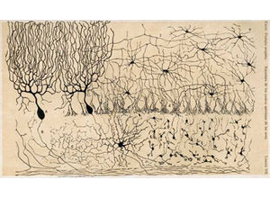
Module12 L3 S02: Where the field started: a hand drawing from sparsely stained tissue, each cell standing alone on a clean background. Set it beside §1.2. rOTO does the opposite on purpose — it puts metal on every membrane in the block, because dense reconstruction needs every boundary — and the price is the crowded field the rest of this unit teaches you to quality-check.
Module12 L3 S06: Two cars joined into one object, with the seam in plain view. That is a merge error you can see. In EM the seam is a membrane too faint for the network to find, which is why §2 prices weak membrane contrast as the expensive artifact: nothing in a summary statistic shows the join.
Module13 L2 S02: One EM field of neuropil. Grade it as §3 asks you to grade every section: are membrane outlines continuous or broken, is there precipitate, is contrast even across the field or does it fall away toward one side? Give anything you find a cost class from the §2 table. (Units 01 and 02 use the same image for scale.)
Module13 L2 S04: A synchrotron, which the source lesson files as tomography context. Non-EM volumetric methods are outside this unit (Unit 02 places them), so use the image for one question only: which rows of the §2 table exist because tissue is cut into sections, and so would not arise in a method that images the block whole?
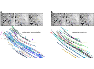
Module13 L2 S09: Automated segmentation (left) against manual annotation (right) of the same processes. Run on a small sub-volume before scaling up, this comparison is the pilot reconstruction §3 calls non-negotiable: count where the automated traces break or fuse relative to the manual ones and you have the split and merge rates your staining produces, while you can still change it.
Lab: acquisition QA report on a real volume (90 minutes)
Setup. Open any public volume in Neuroglancer — MICrONS, FlyWire/FAFB, or H01. Do
not use a curated tutorial view; navigate to arbitrary coordinates.
If you want to see what a whole preparation-and-acquisition chain looks like end to end
before you start, H01, Step by Step
walks one real dataset through every stage in this unit — fixation, ROTO staining, ATUM
sectioning, 61-beam imaging, and the QC that ran during acquisition — with the resulting
micrographs at each scale. It also shows how to pull image data out of a public volume
yourself, which is a faster route to the sampling step below than clicking through the
viewer.
Task. Produce a QA report.
Sample systematically, not conveniently. Choose 10 locations by a rule you
state in advance (e.g. a coarse grid over the volume, or 10 evenly spaced z
sections). Convenience sampling finds clean regions and will make you conclude the
volume is flawless.
At each location, scroll through at least 20 consecutive z sections. Record:
any artifacts from the §2 catalog, membrane contrast on a 1–5 scale with a stated
anchor for each level, and any z-continuity failures.
Classify each artifact as data loss or labor, with a one-line
justification.
Localize. Give coordinates. An artifact report without coordinates cannot be
acted on.
Estimate impact. For each labor-class artifact, estimate the additional
proofreading burden — even crudely (“adds roughly one extra split to fix per
100 µm of axon traced through this region”). State your assumption.
Compute the acquisition budget for this volume from its published voxel size
and extent, using the §1.5 worked example. Compare with the published acquisition
time if you can find it, and explain any discrepancy.
Write three recommendations for a hypothetical next acquisition of the same
tissue, each tied to a specific observation from steps 2–5.
Rubric
Not yet
Proficient
Strong
Sampling
Convenience locations
Stated sampling rule, followed
Rule justified, and coverage bias acknowledged
Identification
“Image looks noisy”
Artifacts named from the catalog
Root cause proposed, with the coordinate-system reasoning that supports it
Cost classification
Absent
Data-loss vs labor assigned
Distribution considered (scattered vs clustered), not just count
Localization
Prose only
Coordinates given
Machine-readable defect list a pipeline could consume
Impact
Not attempted
Qualitative
Quantified with stated assumptions
Recommendations
Generic
Tied to observations
Tied to observations and costed against the tradeoff triangle
Instructor note. Run step 2 as a calibration exercise first: have everyone score
the same three locations, then compare scores publicly before proceeding. Inter-rater
spread on “membrane contrast 1–5” is typically large on the first attempt and shrinks
sharply after one round of discussion. That shrinkage is the learning, and it is
also a live demonstration of why annotation protocols need calibration sessions
(Unit 05).
Common errors and how to recover
Deferring QA until acquisition finishes. Recover: pilot reconstruction, always,
before scaling.
Reporting a single global quality number. Recover: report per-region and
per-section distributions, and always separate data loss from labor.
Chasing SNR instead of contrast. A noisy image with crisp membranes segments
better than a clean image with faint ones. Recover: measure membrane CNR specifically,
not overall image SNR.
Losing the acquisition log. Recover: treat metadata capture as a pipeline stage
with its own tests. If the log is not machine-readable, it does not exist.
Assuming nominal section thickness. Recover: measure it empirically from traced
structures and use the measured value in all geometry.
The norm behind this unit
Some of what this unit teaches is technique. Some of it is professional norm — the
things experienced people do without being asked, and which nobody states out loud
because they assume you already know. Those are worth naming, because they are
distributed unequally by background rather
than by ability.
From this unit:
Separate data loss from labor when you report quality.
One quality score conceals the only distinction the project actually needs. This is the difference between “expensive to fix” and “unanswerable forever”.
Report the distribution, not the count.
Four scattered lost sections and four consecutive lost sections have the same headline number and completely different consequences.
Pilot before you scale.
Running a small sub-volume through the whole pipeline costs 1–2% of a project. Skipping it is the most expensive habit in the field, and no one is ever told to do it explicitly.
The collected set, and why making these explicit is a fairness intervention rather than
etiquette, is in the hidden curriculum.
What this unit does not cover
The alignment and segmentation algorithms that consume this data (Units 04 and 08),
and how to read the biology in a well-prepared image (Units 05–07). It also does not
cover cryo-EM, correlative light-EM workflows in depth, or non-EM volumetric methods
(Unit 02).
Go deeper
Atlas and connectomics reference — the public volumes this unit tells you to open, with access routes and specs in one lookup table
Map at least three artifact types to downstream reconstruction risks.
Define pass/fail QA thresholds before segmentation starts.
Capability development brief
Capability target: Diagnose EM preparation and imaging artifacts and apply QA gates before reconstruction.
Required expertise
EM prep specialist (staining, fixation, section quality)
Imaging engineer (acquisition stability and calibration)
Reconstruction lead (artifact impact on downstream tracing)
Core concepts to teach
Artifact taxonomy: A consistent vocabulary for folds, tears, charging, blur, and alignment distortions.
QA gate: A measurable acceptance threshold required before data moves downstream.
Error propagation: How early imaging defects create false merges or splits later in the pipeline.
Capability exercise
Artifact Triage Lab - Classify artifacts and decide whether blocks pass acquisition QA. The lab above is the graded version of this exercise; do that one.
Assessment artifacts
Annotated artifact atlas with severity labels.
QA checklist with pass/fail thresholds and escalation triggers.
Related concepts
EM Artifacts and QA
Identify acquisition artifacts and define practical QA gates before reconstruction.