Slide 1 of 20
 Nanoscale · Module 14
Computer Vision for EM
Teaching Deck
Human cortex · H01
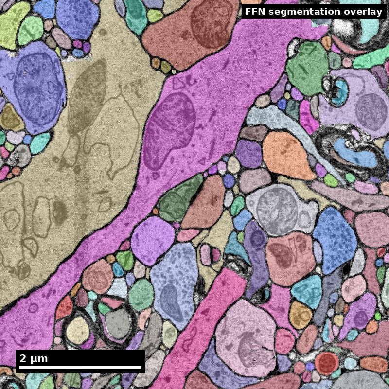
Object segmentation over electron microscopy
H01 release · Lichtman Lab / Harvard & Connectomics at Google · CC BY 4.0
Shapson-Coe et al. (2024) · doi:10.1126/science.adk4858
Slide 2 of 20
Learning Objectives
- Explain how classical and deep CV methods map to connectomics tasks
- Compare model outputs using biologically meaningful error criteria
- Design a validation plan for CV pipelines in EM data
- Report CV limitations with reproducibility safeguards
Slide 3 of 20
Capability Target
Design and evaluate a CV pipeline for EM imagery that is fit for a specific connectomics task and explicitly bounded by known failure modes. Concretely: choose an architecture from the shape of the task rather than from the benchmark leaderboard, decompose error into merges and splits instead of reporting one score, convert that decomposition into a downstream cost using a ratio your team has actually measured, and write a release gate that says in advance what result would stop the model from shipping.
Slide 4 of 20
Concept Focus
1) Task-model fit
- Technical: detection, instance segmentation, denoising, and classification need different objectives, and in EM they also need different data geometry.
Figure description and teaching notes
Further teaching detail from the module:
**Technical:** detection, instance segmentation, denoising, and classification need different objectives, and in EM they also need different data geometry. Affinity prediction with watershed and agglomeration is modular: the dense network runs once over the volume and agglomeration can be re-run cheaply with a new threshold or a learned merge model. Flood-filling networks produce instance labels directly with fewer post-processing stages, at substantially higher compute per volume and less ability to re-run one stage in isolation. Anisotropic data — 4 x 4 x 40 nm is 10:1 — makes z-context weak and pushes some pipelines toward 2D prediction with explicit cross-section linking.
Slide 5 of 20
Concept Focus (continued)
- Plain language: pick the model for the job and for the voxel shape, not by popularity.
- Misconception guardrail: one architecture solves all EM tasks equally well.
Slide 6 of 20
Core Workflow
- Write the EM task as a sentence naming the input, the output, and the downstream consumer of that output.
- Define the acceptable error envelope in decomposed terms: maximum merge rate, minimum ERL, and the region in which those numbers must hold.
- Select a baseline and at most two candidate approaches, using the approach table and the voxel geometry of your data.
- Assemble evaluation data that includes at least one deliberately hard region, and keep clean-region and hard-region metrics separate.
Slide 7 of 20
Core Workflow (continued)
- Evaluate with VI decomposed, ERL, and a connectivity-level metric; never report a single aggregate score alone.
- Convert the error counts into downstream cost using a merge-to-split ratio your team measured rather than assumed.
- Review 20-30 failure cases by eye in ambiguous regions and classify each by cause: weak stain, section loss, fold, thin neurite, or genuine ambiguity.
Slide 8 of 20
Core Workflow (continued)
- Publish a model card with intended use, unsupported uses, the evaluation regions, the metrics with their region breakdown, and the release gate the model passed.
Slide 9 of 20
Run of Show (60 min)
- 00:00-08:00 task framing + exemplar failure modes.
- 08:00-20:00 choose metrics tied to downstream biology.
- 20:00-34:00 evaluate baseline vs candidate model.
- 34:00-46:00 error taxonomy and triage discussion.
Slide 10 of 20
Run of Show (60 min) (continued)
- 46:00-56:00 model card drafting, including at least one unsupported use and the region breakdown of the metrics.
- 56:00-60:00 competency check: each learner states their release gate as a sentence that could fail.
Slide 11 of 20
Misconceptions to Watch
- Misconception guardrail: one architecture solves all EM tasks equally well.
- Misconception guardrail: a higher benchmark score means safer downstream use.
- Misconception guardrail: visual plausibility is sufficient validation.
- Misconception guardrail: the held-out ground truth is representative of the volume.
Slide 12 of 20
Misconceptions to Watch (continued)
- Misconception guardrail: more augmentation is always better than less.
Slide 13 of 20
Studio Activity
Scenario: Compare two segmentation-support CV models for an EM subvolume. You are given the model outputs, a proofread ground-truth subvolume of roughly 40 mm of traced path drawn from a clean region, and a second, smaller ground-truth patch from a region containing a partial fold and two lost sections. Your team maintains the production segmentation and must recommend one model.
Slide 14 of 20
Activity Output Checklist
- Evidence-linked artifact submitted.
- At least one limitation or uncertainty stated.
- Revision point captured from feedback.
Slide 15 of 20
Assessment Rubric
- Minimum pass: clear task-model rationale, biologically relevant metrics reported with merge and split separated, explicit limitations naming at least one unsupported use.
- Strong performance: robust failure analysis by cause, a release gate written before the result was known, and a downstream cost argument that names the merge-to-split ratio as a measured quantity rather than an assumption.
Slide 16 of 20
Assessment Rubric (continued)
- Failure modes: metric-only reasoning, pooling clean and artifact-heavy regions into one number, weak split design, no deployment boundaries, thresholds chosen after seeing which model they would favor.
Slide 17 of 20
Exit Ticket
Document one CV result with one supported use case and one forbidden use case.
Slide 18 of 20
References (Instructor)
- Januszewski et al. (2018) for segmentation model context.
- Recent MICrONS/FlyWire methods for practical CV constraints.
Slide 19 of 20
Teaching Materials
- Module page: /modules/module14/
- Session kit: /teaching/sessions/module14/
- Worksheet: /assets/worksheets/module14/module14-activity.md
Slide 20 of 20
Read, review, or teach
The reading version includes figure descriptions and discussion guidance.
Nanoscale text: CC BY 4.0. Scientific figures retain their individual credits.