Algorithms and Applications

Slide 1 of 58

H01 electron microscopy with object segmentation and original 2 µm scale bar

Algorithms and Applications

Module 9 · EN.585.781 Frontiers in Neuroengineering

Will Gray Roncal · Johns Hopkins University

Part A — Segmentation, error, and the labor problem
Part B — From segmentation to a defensible graph
Part C — Applications, NeuroAI, and what to claim

Human cortex · H01
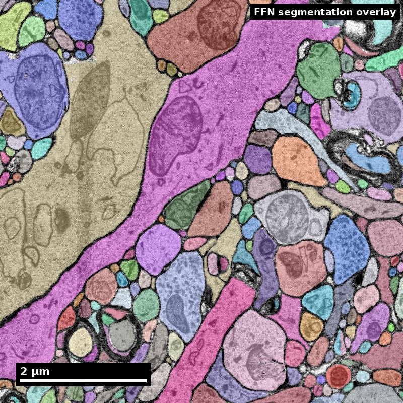
Object segmentation over electron microscopy

H01 release · Lichtman Lab / Harvard & Connectomics at Google
Image: CC BY 4.0 · Shapson-Coe et al. (2024) · doi:10.1126/science.adk4858
Lecture: CC BY-SA 4.0 · neurotrailblazers.org

Figure description and teaching notes

This is the module where the discipline from 7 and the machinery from 8 turn into a
result. The lab is a motif analysis with a defended null model, and the whole of Part B
is aimed at it.

Test 3 covers Modules 7-9. The Bin A/B/C framework and the null-model reasoning are the
two things that will appear in more than one question.

Slide 2 of 58

Where we left off

Module 7 gave you the claim discipline. Bin A / B / C. Scale matching. The non-claim.

Module 8 gave you the instrument. Versioned pipelines, materializations, and the fact that every number is produced by a chain of stages that each fail characteristically.

Module 9 closes the loop.

Voxels → objects → a graph → a claim.

The organizing question all module: what would have to be true for this result to be wrong, and did I check it?

Most of the answers turn out to be about the null model and the error rate — the two things easiest to leave unstated.

Slide 3 of 58

Where Module 9 sits on the discovery pipeline

The last three columns. This is where measurements become claims.

   QUESTION        SPECIMEN         IMAGE           RECONSTRUCTION      GRAPH        CLAIM
      |               |               |                   |              |            |
  measurable      fixation        alignment          segmentation    node/edge      null
   endpoint       staining        ingest             proofreading    definition     model
   null model     sectioning      storage            synapses        inclusion      error band
   non-claim      imaging         serving            versioning      boundary       non-claim
      |               |               |                   |              |            |
   Module 7        Module 8        Module 8        ==== PART A ==== PART B ==== PART B/C ====

Read it right to left when a number surprises you. A motif enrichment that looks too good is, in order of likelihood: a null-model choice (Part B), an inclusion or threshold decision (Part B), a merge-rate problem (Part A), or a version mismatch (Module 8). Only then is it biology.

Slide 4 of 58

Learning objectives

By the end of Module 9 you will be able to:

9.1 — Describe how automated segmentation works and where it fails structurally.

9.2 — Select quality metrics appropriate to a stated endpoint, and explain what each one is blind to.

9.3 — Construct a connectivity graph from a reconstruction, stating every consequential choice.

9.4 — Justify a null model for a stated hypothesis, and interpret a motif result against it.

9.5 — Assess what connectomics and machine learning currently give each other, without overclaiming in either direction.

Slide 5 of 58

Roadmap

Part A — Segmentation, error, and labor How segmentation works, the error taxonomy, the metrics and their blind spots, and the triage discipline that makes proofreading affordable.

Part B — From segmentation to a graph Six construction choices, null models, the triad census, and the error-sensitivity check you should always run.

Part C — Applications and NeuroAI Comparative analysis, cell typing, the results that actually landed, and an honest account of the connectomics/ML relationship.

The lab: a defensible motif analysis. Hypothesis, estimand, null, success criterion, non-claim, provenance. Part B is the preparation for it.

Streams advanced here: 3 — segmentation quality, 6 — structure → function, 4 — modality integration, and 5 — organism coverage via comparative work.

Slide 6 of 58

Part A

Segmentation, error, and the labor problem

How automated segmentation works, and where it fails
The error taxonomy, and why merges are not just "more errors"
Metrics, triage, and stopping rules

Slides 6–21

Slide 7 of 58

The task

Dense instance segmentation, at petascale, where every object is thin and touching

Why this is not ordinary segmentation.

Objects are densely packed with no background — every voxel belongs to something.
Objects are enormous and thin: a single neuron may span millimetres while being 100 nm wide.
There are millions of instances in one volume.
An error at one voxel can change the identity of a millimetre of cable.

The consequence. Segmentation quality cannot be judged per-voxel. A pipeline with 99.99% voxel accuracy can still be useless, because the errors that matter are topological, not areal.

This is why the field's metrics — expected run length, variation of information — are about connectivity of the labeling, not about pixel agreement.

Slide 8 of 58

Two families of algorithm

Affinity + agglomeration. A network predicts, per voxel, the affinity between neighbouring voxels. Watershed at a conservative threshold produces supervoxels that are deliberately too small. An agglomeration step then merges them, using mean affinity, learned agglomeration, or shape descriptors that let the model reason about whether a merge yields a plausible neurite shape.

Strength: parallel, restartable, and the supervoxel layer gives you the immutable atoms Module 8 built everything on.

Flood-filling networks. A network iteratively grows one object from a seed, maintaining a mask and repeatedly asking "does this next voxel belong?"

Strength: the network sees the object it is building, so it has context an affinity model lacks — which is why it produced a step change in accuracy in 2018.

Cost: sequential and expensive.

Januszewski et al. 2018 (10.1038/s41592-018-0049-4, FFN); Funke et al. 2019 (10.1109/TPAMI.2018.2835450, structured-loss affinities); Berning et al. 2015 (SegEM); Nunez-Iglesias et al. 2014 (GALA).

Slide 9 of 58

Ground truth is the scarce resource

Every learned system in this pipeline is limited by densely-labeled tissue that a human made

How it is produced. A skilled annotator densely labels a small volume — every voxel assigned to an object — usually in a tool like VAST or webKnossos. It is slow: a few hundred cubic micrometres is a serious effort.

Why so little exists. The labor is the same labor that proofreads production data, and production always wins the argument for it.

The benchmarks. SNEMI3D and CREMI are the historical public sets. Both are small, both are from specific preparations, and both are old relative to current data.

The consequence you must reason about. A network's reported accuracy is accuracy on tissue like its training set. Change species, staining protocol, section thickness, or microscope, and the number does not transfer.

This is why Module 8's pilot reconstruction matters so much: it measures error on your tissue, which is the only number that predicts your proofreading budget.

Treat any benchmark performance quoted from an older deck or paper as historical context, not as current truth.

Slide 10 of 58

Where both families fail, structurally

These are not bugs. They are consequences of the physics and the data.

Thin processes. A 60 nm spine neck at 40 nm z-resolution may appear in one or two sections. There is very little evidence to work with — spine necks are a perennial source of splits.
Steep z-trajectories. Anisotropy again. A process crossing sections at a shallow angle presents a small, rapidly-moving cross-section.
Membrane contact. Two membranes tightly apposed over many sections may not be separable — especially with weak staining. (Module 8 Part A: this is why understaining is the expensive prep failure.)
Artifact regions. Folds, charging, missing sections. The network was not trained on tissue that does not exist.
Rare morphologies. Anything under-represented in training: unusual cell types, developmental stages, pathology — and, importantly, the boundaries of the volume.

The design choice that shapes everything downstream: the pipeline is deliberately tuned to over-segment. It prefers splits to merges. Therefore proofreading is mostly joining.

Slide 11 of 58

Synapse detection is a separate problem

Why separate. The evidence for a synapse — vesicle cluster, cleft, postsynaptic density — is local and textural. It is not the same signal that separates two membranes, so it gets its own network.

What the output is. A table: coordinates, pre/post supervoxel identity, confidence, cleft size or area.

Partner assignment is its own subproblem. Finding a cleft is easier than deciding which two objects it joins, and getting the direction wrong is a specific, consequential error.

The scoring trap. Synapse precision/recall assumes correct segmentation underneath. A synapse assigned to a merged object scores as correct — the cleft is real and the coordinates are right.

So a pipeline can report excellent synapse metrics while the connectivity it produces is wrong. Synapse-level metrics cannot detect segmentation-level errors. You need both.

SynEM (10.7554/eLife.26414); SyConn (10.1038/nmeth.4206); Synful (10.1038/s41592-021-01183-7); ilastik (10.1038/s41592-019-0582-9).

Slide 12 of 58

The error taxonomy

Error	What it is	Detection difficulty	Cost	Who finds it
Split	One neuron in multiple pieces	Easy — the arbor looks truncated	Bounded, local, visible	Endpoint detectors and humans
Merge	Two neurons fused	Hard — the object looks fine unless morphology is checked	Corrupts connectivity; propagates	Humans noticing implausible morphology
Glia–neuron merge	Glial process fused to a neuron	Hard	High — manufactures local false connectivity	Humans
Orphan fragment	A piece belonging to no traced object	Easy to count	Low individually; large in aggregate as unattributed volume	Automated
False synapse	Detection where none exists	Medium	Inflates degree; worst on 1-synapse connections	Human verification on a sample
Missed synapse	Real synapse not detected	Hard — you are looking for absence	Deflates degree, non-uniformly by synapse size	Human verification on a sample
Wrong partner	Correct cleft, wrong pre/post assignment	Hard	Direction or identity error	Human

Splits are visible and bounded. Merges are invisible and unbounded.

A split leaves evidence of itself — a neuron that stops in mid-neuropil. A merge leaves an object that looks like a neuron and is not. The whole architecture of the field — watershed thresholds, proofreading protocols, quality metrics — is organized around this asymmetry.

Slide 13 of 58

Automated error detection: where the leverage is

The proofreading bottleneck is a detection problem before it is a correction problem

Split candidates are comparatively easy. A neurite that stops without tapering to a natural ending is suspicious, and an endpoint detector finds them cheaply. This is why splits are the manageable error even at scale.

Merge candidates are the hard, valuable case:

Morphology implausibility — two somata in one object; an object carrying both ribosome-rich cytoplasm and presynaptic vesicle clusters
Cue conflict — axonal and dendritic evidence in the same continuous object
Agglomeration confidence — low-confidence joins, surfaced for review
Learned error detection — a network trained to spot segmentation mistakes rather than to segment

Why this is the highest-leverage open problem in the module.

Every hour of human attention saved multiplies across every dataset in the field, and the 500× to a whole mouse brain is unreachable without it.

It is also unusually tractable for a student project: the inputs are public, the evaluation is well-posed, and a modest improvement is immediately useful to real projects.

Slide 14 of 58

Metric	Measures	Blind to	Use when
Variation of Information (VI)	Total disagreement between two segmentations, decomposable into split and merge components	Object size — merging two tiny fragments and merging two full neurons contribute very differently, and not in the way you want	Comparing segmentation versions on the same volume
Expected Run Length (ERL)	Mean error-free path length along skeletons	Merges, unless explicitly penalized; also small dangling fragments	"How far can I follow a neurite before hitting an error?"
Edge precision / recall	Correctness of connections in the derived graph	Weights all edges equally — a 1-synapse and a 50-synapse connection count the same	Graph-level claims
Synapse precision / recall	Correctness of detected synapses	Assumes correct segmentation underneath	Synapse-level claims
Completeness (per neuron)	Fraction of a neuron actually reconstructed	Says nothing about correctness of what is there	Per-cell claims like input counts

Use at least two metrics from different rows, and always report VI's split and merge components separately. A single VI number can improve while merges get worse, because the split component dominates. That is a real and common way to ship a regression.

Slide 15 of 58

Check yourself

Version B has lower total VI than version A. Your team wants to ship it. What do you check first?

Decompose VI into split and merge components.

Total VI is dominated by whichever component is larger, and in an over-segmented pipeline that is usually splits. Version B may have reduced splits — perhaps by more aggressive agglomeration — while increasing merges. The total still improves.

Since merges are the expensive error, a better total VI with worse merges is a regression for connectomics purposes, even though the headline number improved.

Then check two more things:

ERL — does tracing actually get easier? A metric that measures the thing proofreaders experience.

The endpoint metric, recomputed on a fixed evaluation set of neurons. Decisive.

Ship on the endpoint, not on the aggregate score.

Slide 16 of 58

The metric that actually matters is none of them.

It is the effect on your endpoint.

If your result is "cell type A makes 3× more synapses onto B than onto C", the question is not "what is our VI?"

It is: how much would the observed 3× change under a plausible correction of the remaining errors?

Slide 17 of 58

The highest-value practice in this module

Quantify your own error, on your own endpoint, with about forty person-hours

Take a random sample of the cells in your analysis — 20 is often enough to be informative.
Proofread them exhaustively, to a standard well above your production standard.
Recompute the endpoint on that sample, before and after.
Report the shift.

"Exhaustive proofreading of a 20-cell sample changed the ratio from 3.1 to 2.8."

That is a far stronger statement about data quality than any VI value, and reviewers understand it immediately. It converts "we proofread the data" into a quantified error bound.

Note what makes it work: it is a differential measurement on the quantity you actually report — so it needs no assumption about how VI maps onto your endpoint.

Slide 18 of 58

The production proofreading loop

1. SEED       Select target cells by scientific priority — not by convenience,
                and not by which segment happens to be biggest.

2. TRIAGE     Rank candidate corrections by expected effect on the endpoint.

3. CORRECT    Apply merges and splits with the evidence recorded.

4. VERIFY     Independent second pass on a sample; measure agreement.

5. MEASURE    Recompute quality metrics AND the endpoint metric.

6. STOP       Apply the stopping rule. Record the state as a release.

Step 1 is where most projects go wrong before they start. "Proofread the biggest segments" is a convenience heuristic that systematically over-samples large cells — which correlates with cell type, position, and completeness. You will have conditioned your analysis on a variable you never named.

Slide 19 of 58

Triage: rank by endpoint change per annotator-minute

Not by how conspicuous the error is

Proximity to the endpoint. An error on a cell in your analysis set outranks an identical error on a cell that is not.
Error type. Merges outrank splits at equal size, because merges corrupt rather than truncate.
Size. A split that truncates 60% of an arbor outranks one losing a 3 µm twig — but note that a small merge can be worse than a large split, so size ranks within type, not across types.
Path centrality. An error on the primary neurite near the soma disconnects everything distal to it. Errors near the root are worth far more than errors at the tips.
Cost to fix. A 40-minute correction through a fold may lose to five 5-minute corrections elsewhere.

Automated candidate generation feeds the queue: endpoint detectors (a neurite that stops without tapering), morphology-implausibility detectors (two somata in one object), agglomeration-confidence thresholds. Humans adjudicate a ranked queue rather than browsing.

Slide 20 of 58

Worked example: three candidates, one annotator-hour

Setup. The study needs 200 proofread L2/3 pyramidal cells for a cell-type targeting endpoint. The queue's top three, with one hour available:

A — a split: an analysis-set cell's primary apical dendrite truncated near the soma, detaching ~60% of the arbor. Fix: 10 min.
B — a glia–neuron merge: a fine astrocytic process fused onto another analysis-set cell's basal dendrite. Fix: 20 min.
C — a conspicuous merge: two somata in one object, flagged by the detector. Neither cell is in the analysis set. Fix: 15 min.

Proximity. A and B sit on analysis-set cells. C looks dismissible — but not yet. C could corrupt the endpoint indirectly, if either fused neuron is presynaptic to an analysis cell, because the merge scrambles the presynaptic identity of those inputs. Check the partner lists — two minutes — and find no synapses onto the 200. Only now does C drop.

The assumption "C does not touch the endpoint" has been tested, not presumed. Two minutes of checking is part of the triage, not overhead.

Slide 21 of 58

Worked example, resolved

Error type. B corrupts: the astrocytic path drags past synapses the dendrite never contacted, and those false inputs enter the class fractions silently. A truncates: the input count is undercounted, but visibly — the cell fails the "dendrite complete" criterion and is excluded until fixed.

An unfixed A delays a cell. An unfixed B poisons one.

Size and centrality. Within splits, A is severe — near the root, most of the arbor detached. But size ranks within type: A's 60% does not outrank B's merge.

Cost. A is half B's price. Per expected endpoint change per minute, B still wins: removing silent corruption beats accelerating a visible, bounded repair.

The hour. B (20) + A (10) + the partner check on C (2) = 32 minutes. The remaining 28 do not go to C — its only argument was conspicuousness, which is not a factor — but to the next analysis-set candidates, roughly five more corrections at a five-minute median. C is logged with a reason, unfixed.

Slide 22 of 58

Stopping rules

Where most projects fail, because "keep going until it looks good" has no termination condition

Rules that work, because they can be satisfied and reported:

Endpoint stability. Stop when an additional k annotator-hours shift the endpoint by less than a stated tolerance.
Sampled agreement. Stop when independent second-pass agreement on a random sample exceeds a stated threshold.
Budget with disclosure. Stop at a fixed budget and report the residual error rate you measured.

Rules that do not work:

"Until it looks good" — unfalsifiable, and biases toward the analyst's expectation
"Until VI is below x" — optimizes an aggregate, not your claim
"Until we run out of time" — fine as a constraint, useless as a rule, and disastrous when undisclosed

Record the stopping state as a release (Module 8), so analyses can cite it.

Slide 23 of 58

Part A checkpoint — human factors, because this is a labor operation

Proofreading is the dominant project cost. That makes it a management problem, not only a tooling one:

Training and calibration. Annotators drift. Periodic calibration on a gold-standard set catches it before it enters the data.
Inter-annotator agreement, measured routinely — not once at the start.
Task design. Ranked queues beat free browsing; short focused tasks beat open-ended ones.
Retention. Experienced annotators are much faster and more accurate. Turnover is a data-quality risk.

Community proofreading (EyeWire 2014, FlyWire 2024) is the field's most successful answer so far: it changes who can contribute and how the work scales.

It also introduces its own quality-management problem — consensus mechanisms, reputation weighting, and adjudication — which is a research area in its own right.

Break. Part B: turning a proofread reconstruction into a graph you can defend.

Slide 24 of 58

Part B

From segmentation to a defensible graph

Six consequential construction choices
Null models: choosing the null is the scientific step
Motifs, error sensitivity, and what lies beyond

Slides 22–39

Slide 25 of 58

Graph construction is a sequence of consequential choices

Six decisions. Each changes the answer. Each must be stated.

1 — What is a node? A cell? A cell type? A compartment? Cell-type nodes give more power and less resolution. Compartment-level nodes (soma, proximal dendrite, distal dendrite, AIS) preserve information most analyses discard — and that is often where the biology lives.

2 — What is an edge? A single detected synapse is usually a poor edge: 1-synapse connections are the least reliable part of the data, most vulnerable to false-positive detection and to merge errors. Common practice thresholds at ≥ 2 or ≥ 3.

3 — Weighted or binary? Synapse count is the usual weight. Contact area or total PSD area is arguably a better strength proxy and is available in modern datasets. Binary is defensible for topological questions and discards real information otherwise.

Slide 26 of 58

Three more, and the one that is least reported

4 — Direction. Retained, derived from the axon/dendrite call — with all the caveats about direction errors that come with it.

5 — Inclusion criteria. The highest-leverage and least-reported decision.

If you include only well-proofread cells, you have conditioned on a variable correlated with cell size, position, and type. If you include everything, you have mixed completeness levels.

Either is defensible. Neither is defensible silently.

6 — Boundary handling. Cells cut by the volume edge have truncated arbors and undercounted partners. Either restrict to cells whose relevant arbor is fully contained, or model truncation explicitly. Doing neither produces a spatial gradient in apparent connectivity that follows the shape of the volume — and looks like biology.

Slide 27 of 58

The synapse threshold is not innocent

Thresholding at ≥ 2 or ≥ 3 synapses removes a large fraction of edges — the synapses-per-connection distribution is heavy-tailed, and single-synapse connections typically dominate by count.

Worse, it removes them non-uniformly across cell types, because some types genuinely connect via few synapses.

The rule. Always report the threshold, and always re-run the headline result at a second threshold.

If the conclusion flips, that is the finding. Report it as such rather than choosing the threshold that produced the tidier story.

Your graph has 400 nodes and 5,000 edges. Your collaborator's, from the same dataset, has 400 nodes and 1,800 edges. Neither of you made an error. How?

Figure description and teaching notes

Most likely the synapse threshold: at >=1 you keep every detected connection, at >=3 a
minority. Given the heavy tail, 1 -> 3 can easily remove more than half the edges.

Other candidates worth surfacing: different materialization versions (Module 8 --
proofreading continued between the two queries); different inclusion criteria; different
boundary handling; different synapse-confidence cutoffs.

The lesson is procedural, and say it explicitly: graph construction must be a VERSIONED
ARTIFACT with recorded parameters, not a script someone ran once. "How many edges does
your graph have?" is a question about parameters, not about biology.

Slide 28 of 58

Read these basic statistics before any motif

They shape every null model you will choose, and they catch construction errors early

Degree distribution. Heavy-tailed, essentially always. A few hub cells with very many partners; a long tail with few. This is why Erdős–Rényi is the wrong null — and why degree-preserving rewiring is the minimum defensible baseline.

Synapses-per-connection distribution. Also heavy-tailed, with single-synapse connections usually dominating by count. This is why the edge threshold is so consequential.

Connection probability vs distance. Falls steeply. Plot it before choosing a null; if you cannot estimate this curve, you cannot use a distance-preserving null honestly.

Use them as a construction check, not just description.

A degree distribution with an implausible right tail often means merges. A synapse count that jumps when you change materialization version means you queried latest. A connectivity gradient that follows the volume's shape means boundary handling was skipped.

Each of these is visible in a plot you can make in five minutes, and invisible in the motif result you would otherwise publish.

Slide 29 of 58

A motif is "enriched" only relative to a null.

The null encodes what you consider uninteresting.

Choosing the null is the scientific step. Running the test is bookkeeping.

Write out, in words, the sentence "it would be uninteresting if this pattern arose merely because ___." If you cannot finish that sentence, you do not yet know what you are testing.

Slide 30 of 58

Null models

Null model	Preserves	Appropriate when	Danger
Erdős–Rényi	Node count, edge count	Almost never for connectomes	Ignores degree heterogeneity; will show "enrichment" of nearly every motif
Configuration / degree-preserving	In- and out-degree of every node	Testing structure beyond degree	Does not control for space or cell type
Distance-dependent	Degree + the empirical connection-probability-vs-distance curve	Spatially embedded data — i.e. all volume EM	Requires estimating the distance curve, which is itself error-prone
Cell-type-preserving	Type-to-type connection probabilities	Testing structure beyond type identity	Requires reliable cell types
Generative / latent-position	A fitted low-dimensional structure	Testing residual structure	The model can absorb the effect you are looking for

The rule: preserve everything you are not asking about.

If the hypothesis is "reciprocity exceeds what degree and distance explain", the null must preserve degree and distance. Otherwise you have measured degree heterogeneity and spatial proximity, and called it a motif.

Slide 31 of 58

Worked example: reciprocity, under three nulls

Hypothetical graph: 100 neurons, 1,200 directed edges, 210 reciprocal pairs

Null 1 — Erdős–Rényi. Edge probability p = 1200 / (100 × 99) = 0.121.

E[recip] = p^2 x N(N-1)/2 = 0.0147 x 4,950 = 72.7

observed / expected = 210 / 72.7 = 2.9x

A 2.9-fold enrichment under this model. The ratio alone is not a test result.

This independent-edge model fixes the expected edge count, not its exact value. It does not preserve node degrees, distance or cell type. A fixed-edge-count null is a different model.

Slide 32 of 58

Worked example, null 2 — degree-preserving

Two high-degree cells are much more likely to connect in both directions by chance alone. So preserve each node's in- and out-degree, rewire 10,000 times, and count reciprocal pairs each time.

Suppose the null distribution has mean 150, sd 12:

observed / expected = 210 / 150 = 1.4x
z = (210 - 150) / 12            = 5.0

The ratio falls from 2.9× to 1.4×. The z-score is descriptive; a tail probability requires the null distribution or an explicit distributional assumption.

These null summaries are illustrative, not measured. Changing the constraints changes the comparison; it does not establish a causal contribution of degree heterogeneity.

Slide 33 of 58

Worked example, null 3 — degree and distance

Connection probability falls steeply with inter-somatic distance, and reciprocal partners are disproportionately near neighbours. Rewire preserving both degree and the empirical distance–probability curve. Suppose mean 185, sd 14:

observed / expected = 210 / 185 = 1.14x
z = (210 - 185) / 14            = 1.8

Test direction matters. A normal approximation gives p ≈ 0.074 two-sided, but ≈ 0.037 for a prespecified upper tail. Do not choose the direction after seeing the result.

An enrichment ratio does not determine significance. For a real analysis, estimate the tail from a validated null sampler and state the direction, decision rule and multiplicity treatment.

Pre-register the null, or at minimum report the result under all three.

Slide 34 of 58

"But the distance null throws away the biology"

A real objection. The resolution is that it depends on the hypothesis.

"Is there specific reciprocal wiring beyond generic spatial and degree structure?" → Distance must be controlled. Spatial proximity is exactly the alternative explanation you are trying to exclude.

"Is reciprocity higher in circuit X than circuit Y?" → A distance-preserving null within each circuit may over-control. If the two circuits differ in their distance dependence, that difference is part of what you are measuring.

"What generates the observed reciprocity?" → Not a single null at all. Compare generative models: fit distance-only, distance-plus-type, and distance-plus-type-plus-reciprocity-bias, and compare fit with a complexity penalty.

The general principle. The null is a statement of what would count as an uninteresting explanation. Write that sentence in words before choosing one.

Slide 35 of 58

Motif analysis: the triad census

16 isomorphism classes of directed three-node subgraphs. Count them; compare to a null.

Four things that go wrong:

1 — Multiple comparisons. Testing all 16 classes means 16 tests. At α = 0.05 you expect roughly one false positive by chance. Correct for it — Bonferroni is conservative but defensible at 16; Benjamini–Hochberg if you prefer FDR. Report how many tests you ran, including the ones you did not report.

2 — Non-independence. Triad counts are strongly correlated — adding one edge changes many triads at once. Treating the 16 as independent overstates confidence. This is a strong argument for permutation-based inference, which respects the dependence naturally.

Slide 36 of 58

The third failure is the one that will get you

Merge-error bias is not symmetric

A merge combines partner lists, but can also collapse duplicate edges or turn an edge into an excluded self-loop.

The direction depends on the motif and construction rules. Combining two disjoint partner lists alone does not create triangles without connections among the partners.

Splits can remove or redistribute edges and change which motif class a subgraph occupies.

Do not assume cancellation or a universal direction.

Construct explicit error scenarios and recompute the endpoint. Unvalidated segmentation is not automatically conservative.

4 — Cell-type confounding. If types A and B are both numerous and preferentially interconnect, triads with two A's and one B are over-represented — a type-composition effect, not a wiring motif. Use a type-preserving null, or analyze within type.

Slide 37 of 58

The error-sensitivity check you should always run

A few dozen lines of code, and one of the strongest things you can put in a supplement

State your estimated merge and split rates — from the Part A validation sample, not from a paper about a different dataset.
Specify an error model. Perturb identities or edges using mechanisms supported by validation. Rates alone do not specify which objects are likely to be wrong.
Recompute the motif statistic on many such perturbed graphs.
Report the resulting spread as a sensitivity band, conditional on that error model. It is not automatically a calibrated confidence interval.

If plausible perturbations reverse the result, report that sensitivity. Recompute the matching null when graph properties change. Robustness to a chosen error model is not proof of correctness.

Notice how Parts A and B just joined: the Part A resample gives you the rates, and this check turns them into an error bar on the Part B claim. Neither half is useful alone.

Slide 38 of 58

Multiple testing and pre-registration, in practice

The garden of forking paths is wide here. Between raw data and a motif p-value sit: the materialization version, the synapse threshold, the confidence cutoff, the inclusion criteria, the boundary rule, the node definition, the null model, and the test. Each has several defensible settings.

Analysts do not usually cheat. They try a reasonable setting, get an unclear result, try another reasonable setting, and report the one that worked. The p-value does not know that happened.

What actually helps, in ascending order of effort:

1. Report every test you ran, including the unreported ones. 2. Fix the analysis parameters before looking at the outcome, and say when you fixed them. 3. Split the data: explore on one half, confirm on the other. 4. Pre-register the hypothesis, null, and success criterion. Cheap in this field, because the datasets are public and stable.

Keep exploratory and confirmatory analyses explicitly separated in the write-up. Exploration is legitimate and valuable — mislabeling it as confirmation is not.

Slide 39 of 58

Beyond motifs

Community detection. Modularity methods have a known resolution limit — they cannot find communities below a size that depends on the graph — and they return a partition for any graph, including a random one. Always compare obtained modularity against degree-preserving rewired graphs.

Spectral embedding and latent-position models. Represent each node as a point in a low-dimensional space fitted from adjacency. Useful for cell typing from connectivity and for comparing graphs. Careful with sparse and directed graphs: the adjacency spectral embedding of a directed graph is not the same object as that of its symmetrized version.

Graph matching. Finding the correspondence between two connectomes — left versus right hemisphere, or two individuals. Computationally hard in general; usable approximations exist and have been applied to bilateral matching in the larval Drosophila connectome. The payoff is a measure of how stereotyped wiring is — a question only connectomics can answer.

Cell typing from connectivity. Cluster cells by connectivity profile; ask whether the clusters agree with morphological or transcriptomic types. When they disagree, that is interesting — and should not be resolved by quietly picking the answer you prefer.

Slide 40 of 58

Part B checkpoint — the graph provenance block

What must accompany every connectomics graph you publish

dataset:              minnie65_public
materialization:      943
node_definition:      proofread pyramidal cells, L2/3, soma in volume
edge_definition:      synapse_count >= 3, direction from axon/dendrite call
weighting:            synapse count (contact area archived)
inclusion_criteria:   dendrite completeness >= 0.8; axon not required
boundary_handling:    cells with >10% arbor outside volume excluded (n=17)
n_nodes:              412
n_edges:              5,003
threshold_sensitivity: re-run at >=1 and >=5; conclusion stable (see S3)
null_model:           degree- and distance-preserving, 10,000 rewires
error_rates:          merge 0.8%, split 4.1% (20-cell exhaustive resample)

Eleven lines. They pre-answer nearly every methodological question a reviewer can ask, and they take ten minutes. The lab requires this block.

Slide 41 of 58

Part C

Applications, NeuroAI, and what to claim

Comparative analysis and cell typing
Three results that actually landed
What connectomics and machine learning give each other

Slides 40–56

Slide 42 of 58

Comparative and developmental analysis

Where several of the field's most durable results have come from

Why comparison is stronger than measurement. A comparison controls for many reconstruction biases that a single measurement cannot. If both connectomes were reconstructed by the same pipeline with the same error rates, a difference between them is far more robust than either absolute value.

Across development. The C. elegans series (Witvliet et al. 2021) across eight stages: which connections are stable through maturation, and which are added.

Across sexes. Fly male and female CNS releases (2024–25): sexual dimorphism at connectome scale, in the same species with the same tooling.

Across hemispheres. Bilateral matching in the larval Drosophila connectome measures stereotypy — how much of wiring is specified rather than idiosyncratic.

Across species. Octopus vertical lobe, Ciona, Platynereis, zebra finch. A learning circuit that evolved independently is the strongest available test of which architectural features are necessary rather than historical.

Slide 43 of 58

Cell typing: three definitions that should agree

Morphological — shape, arborization, laminar position. The oldest definition, and the one EM delivers directly.

Transcriptomic — expression profile. High-resolution, and now the field's default census for many regions — but no geometry and no connectivity.

Connectivity-based — cluster cells by who they connect to. What a connectome uniquely offers.

When they agree, you have converging evidence for a type — which is a much stronger claim than any one method supports alone.

When they disagree, that is a finding. It may mean a transcriptomic type contains connectivity subtypes, or that a morphological class is not a functional unit.

What not to do: resolve the disagreement by quietly picking the answer you prefer, or by relabeling until the methods agree. The disagreement is data.

Slide 44 of 58

Three results that actually landed

1 — Retinal direction selectivity. Reconstruction showed that starburst amacrine inhibition onto direction-selective ganglion cells is organized by space–time wiring specificity — a structural asymmetry that predicts the computation. Structure gave the mechanism; physiology confirmed it.

2 — The fly central complex as a ring attractor. The connectome revealed a ring of heading-tuned cells with the recurrent and inhibitory architecture a ring attractor requires. The theory pre-existed; the wiring turned it into a specific, testable claim about identified cells.

3 — Connectome-constrained models (Lappalainen et al. 2024). Fix a network model's connectivity to the measured fly visual connectome, fit only the remaining parameters — and the model predicts neural responses that were then tested.

Read the pattern. In all three, the connectome removes free parameters and turns a vague hypothesis into a falsifiable one.

That — not simulation — is what a wiring diagram is for.

Slide 45 of 58

What a connectome-constrained model actually is

Worth unpacking, because the phrase gets used loosely

The construction, concretely:

Take the measured connectome. Fix the model's connectivity matrix to it — which neurons connect to which, and how strongly, by synapse count.
Leave free what the connectome cannot specify: sign, time constants, gains, nonlinearities.
Fit those free parameters to a task or to recorded data.
Predict responses the fitting never saw, and test them.

Why this is a strong design. Fixing connectivity removes an enormous number of free parameters. A model with fewer free parameters that still predicts held-out data is doing more work per assumption — and it can fail, which is the point.

Where it is fragile. The connectome fixes topology, not weights. Step 2 quietly re-introduces sign and gain as free parameters — so the model can sometimes compensate for a wrong topology by fitting those. Ask what happens when the connectivity is shuffled: if performance barely drops, the connectome was not doing the work.

Lappalainen et al. 2024, 10.1038/s41586-024-07939-3 — fly visual system.

Slide 46 of 58

NeuroAI: two symmetric errors to avoid

Error 1 — dismissing the connection. "Connectomics has contributed nothing to machine learning."

Too strong. Connectome-constrained models are a real and growing result type, and connectomics has generated genuinely hard ML problems whose solutions transferred.

Error 2 — overselling it. "The connectome will give us the brain's algorithm."

Also too strong, and much more common in talks. It confuses a constraint on the space of dynamics with the dynamics.

This section exists to let you hold both at once. The accurate position is specific, defensible, and slightly boring — which is usually the sign that it is right.

Slide 47 of 58

What connectomes give machine learning today

Constraints for network models. The strongest current result type. Take a measured connectome, use it to fix a dynamical model's connectivity, fit the remaining parameters to data, and predict neural responses. Done in the fly visual system, where predictions were then tested.

The connectome is doing real work here. It removes an enormous number of free parameters — which is exactly what makes the model falsifiable.

Architectural priors, honestly scoped. Measured circuit motifs — specific recurrence patterns, canonical microcircuit structure, the ring architecture of the central complex — can inspire architectures. The honest framing is inspiration plus hypothesis, not derivation. Very few production ML systems trace a design decision to a connectome.

Benchmarks and hard problems. Petascale dense segmentation, few-shot generalization across tissue preparations, error detection in structured outputs. Progress on these has been real and transferable.

Slide 48 of 58

What connectomes do not give machine learning

Not weights. Synapse count is a proxy for strength, not a synaptic weight. Sign, short-term dynamics, plasticity state, and neuromodulatory context are all absent.
Not dynamics. A static wiring diagram, from one animal, at one moment.
Not a runnable brain. Uploading or simulating a connectome directly is not on the near horizon, and saying so plainly is part of doing this work credibly.
Not, so far, a competitive advantage in mainstream deep learning. The architectures that dominate practice were not derived from neuroanatomy.

Each of these is a Bin C statement from Module 7, arriving from the other direction. The wiring diagram constrains; it does not specify.

Slide 49 of 58

The reverse direction is currently much stronger.

Machine learning has contributed far more to connectomics than the reverse.

Dense segmentation, synapse detection, error detection, automated proofreading candidate generation — all learned systems. None of the petascale datasets would exist without them.

When you write about NeuroAI, note the asymmetry. It is the accurate description of the present state, and it costs nothing to be right about.

Slide 50 of 58

Open problems worth a thesis

Automated error detection at scale. The proofreading bottleneck is a detection problem: find the merges without a human looking at everything. Every hour saved here multiplies across the field.

Cross-individual variability. Almost every landmark dataset is n = 1. Which features are stereotyped and which idiosyncratic is largely unmeasured.

Molecular identity at scale. Bridging EM geometry to transcriptomic type — CLEM, expansion, barcoding. Open and active.

Connectome-constrained models beyond the fly. The Lappalainen result is a template. Whether it transfers to mammalian cortex, where the volume is a fragment of the circuit, is unknown.

Comparative connectomics. Under-occupied relative to its yield, and tractable at volumes far below a mouse mm³.

Statistical methods for connectomes. Sparse, directed, spatially embedded, error-laden graphs with n = 1. Most of network science assumes away at least three of those.

Slide 51 of 58

The eight streams, revisited

Where each one stands, and what would move it next

Stream	The result that defines it today	What moves it next
1 · Scale	1 mm³ mouse and human volumes; whole adult fly brain	Whole mouse brain — ~800 PB, and an engineering program, not a microscope
2 · Throughput and automation	Multibeam SEM; FAST-EM; SmartEM's adaptive dose	Unattended alignment; proofreading hours per mm of cable falling
3 · Segmentation quality	Flood-filling networks; learned agglomeration	Automated merge detection — the highest-leverage open problem in this module
4 · Modality integration	MICrONS: EM co-registered with two-photon function	Molecular identity at scale — CLEM, expansion, barcoding
5 · Organism and lifespan	C. elegans developmental series; fly male and female CNS	Cross-individual variability; almost every landmark dataset is n = 1
6 · Structure → function	Connectome-constrained models predicting fly visual responses	The same argument in a mammalian volume that holds only a fragment of the circuit
7 · Openness and community	EyeWire; FlyWire community proofreading; BossDB, neuPrint, CAVE	Quality management for distributed proofreading; egress economics
8 · Translation and people	H01 human cortex; brain banking; training programs	Health links that survive the n = 1 and clinical-provenance caveats

Use this as a placement exercise, not a summary. Take the last connectomics paper you read and put it in a row. If it does not fit one, either you have found something genuinely new — or the paper is advancing a stream it did not declare.

Slide 52 of 58

Communicating this work without overclaiming

Weak

"We reverse-engineered a brain circuit."

"The connectome shows how the brain computes."

"This is a complete map of the human cortex."

"AI cracked the connectome."

Defensible, and more interesting

"We measured the wiring of an identified circuit and used it to constrain a model that predicted responses we then tested."

"The connectome narrows which computational models are consistent with the anatomy."

"~1 mm³ of human temporal cortex, surgical resection, n = 1."

"Learned segmentation made a petascale reconstruction affordable; proofreading remains the dominant cost."

Every right-hand phrasing is shorter on certainty and longer on information. For public audiences, that trade gains interest rather than losing it — a real constraint honestly described is a better story than a vague triumph.

Slide 53 of 58

Ethics, provenance, and dual use

Human tissue carries obligations that travel with the data. Consent frameworks, de-identification, IRB conditions, and the clinical context of the sample. State them in the dataset record and in the results — not in the supplement.

And provenance is interpretive, not administrative. H01 is tissue from a patient with epilepsy. Any claim about "the human cortex" from that sample must reckon with the clinical history, the medication, and the resection margin. "Human temporal cortex (surgical resection, epilepsy)" is the honest noun phrase.

On "mind reading" and "uploading." Both come up whenever this work reaches a general audience, and both deserve a plain answer: a static wiring diagram from fixed tissue contains no dynamics, no plasticity state, and no neuromodulatory context. Simulating or uploading a connectome is not on the near horizon.

Saying that clearly is not modesty; it is credibility. A field that lets its popular framing outrun its evidence spends the difference later, and the people who pay are the students entering it.

Slide 54 of 58

The lab: a defensible motif analysis

Two hours. The graded artifact for Module 9.

Produce one analysis card with every field filled:

Field	What it must contain
Hypothesis	One sentence, in words, falsifiable
Estimand	The quantity being estimated, with units
Graph construction	The eleven-line provenance block from Part B
Null model	Named, with the "it would be uninteresting if…" sentence written out
Success criterion	Stated before running anything
Error sensitivity	Effect size with a band from your measured merge/split rates
Non-claim	What these data do not establish
Provenance	Dataset, materialization version, code revision, seed

Rubric weighting. A coherent hypothesis–null–estimand chain passes. Sensitivity analysis and a boundary statement make it strong. A result-first narrative without methodological controls is flagged, however clean the figure.

Slide 55 of 58

Module 9 assignment and Test 3

Module assignment. Five short-answer questions: a metric-choice justification; a triage ranking with reasoning; a graph-construction critique; a null-model selection; and an error-sensitivity interpretation.

Discussion forum. Find a published connectomics claim you think is one bin too strong. Quote it fairly, say which bin it belongs in and why, and name the additional measurement that would justify the stronger claim.

Test 3 covers Modules 7–9. The two things that recur across questions:

1. The Bin A / B / C sort, applied to unfamiliar claims.

2. Null-model reasoning — given a hypothesis, name what the null must preserve, and why.

Everything else is a specific instance of one of those two.

Slide 56 of 58

Where to go next

If you want to do this work. Open a public volume this week — neuPrint, FlyWire Codex, or CAVE — and reproduce one figure from a paper. Nothing else teaches the gap between a published number and a queryable dataset as fast.

If you want to build tools. The error-detection and triage problems in Part A are open, tractable, and immediately useful to everyone in the field.

If you want to model. Read Lappalainen et al. 2024, then ask what it would take to run the same argument in a mammalian volume where you can only see a fragment of the circuit.

The one idea to carry out of all three modules.

A connectomics result is a measurement — with a stated sampling, a stated error rate, and a stated non-claim.

Everything else is illustration.

Slide 57 of 58

References and sources

Segmentation and proofreading. Januszewski et al. 2018 (10.1038/s41592-018-0049-4, flood-filling networks); Funke et al. 2019 (10.1109/TPAMI.2018.2835450, structured-loss affinities); Berning et al. 2015 (10.1016/j.neuron.2015.09.003, SegEM); Nunez-Iglesias et al. 2014 (10.3389/fninf.2014.00034, GALA); Helmstaedter et al. 2011 (10.1038/nn.2868, RESCOP consensus); Kim et al. 2014 (10.1038/nature13240, EyeWire); Dorkenwald et al. 2024 (FlyWire community proofreading); Dorkenwald et al. 2025 (10.1038/s41592-024-02426-z, CAVE).

Synapse detection. Staffler et al. 2017 (10.7554/eLife.26414, SynEM); Dorkenwald et al. 2017 (10.1038/nmeth.4206, SyConn); Buhmann et al. 2021 (10.1038/s41592-021-01183-7, Synful); Berg et al. 2019 (10.1038/s41592-019-0582-9, ilastik).

Graph analysis. Milo et al. 2002 (10.1126/science.298.5594.824, network motifs); Bates et al. 2020 (10.7554/eLife.53350, natverse); Winding et al. 2023 (larval CNS graph and bilateral matching); Bassett, Zurn & Gold 2018 (model taxonomy and claim types).

Applications and modeling. Briggman et al. 2011 (retinal direction selectivity); Kim et al. 2014 (space–time wiring specificity); Scheffer et al. 2020 (10.7554/eLife.57443, hemibrain); Dorkenwald et al. 2024 (FlyWire); MICrONS Consortium 2025 (10.1038/s41586-025-08790-w); Lappalainen et al. 2024 (10.1038/s41586-024-07939-3, connectome-constrained networks); Abbott et al. 2020 (10.1016/j.cell.2020.08.010, "The Mind of a Mouse").

Course material. NeuroTrailblazers technical training Units 08, 09.
https://neurotrailblazers.org

Slide 58 of 58

Use, adapt, and credit

These slides are openly licensed for community use

Licence: CC BY-SA 4.0
Creative Commons Attribution-ShareAlike 4.0 International.
https://creativecommons.org/licenses/by-sa/4.0/

You may teach from these slides anywhere, including commercially; copy and redistribute them in any medium; and re-cut, shorten, translate, restyle, or merge them into your own material — and distribute the result. No permission needed.

Two conditions. Attribution — credit the original, link the licence, and say if you changed anything. ShareAlike — distribute your adapted version under this same licence, so it stays as open as what it came from.

How to credit

Gray Roncal, W. (2026). Nanoscale Connectomics: Algorithms and Applications (EN.585.781 Frontiers in Neuroengineering, Module 9). NeuroTrailblazers. CC BY-SA 4.0. neurotrailblazers.org/teaching/lectures/

For an adaptation, prefix with "Adapted from" and note what you changed.

Editable source. The Marp markdown is in the repository — the exported PowerPoint renders each slide as an image, so the markdown is the thing to edit. https://github.com/wrgr/neurotrailblazers

Improved something? The project would like to hear about it — open an issue.

Cover image: H01 release, Lichtman Lab / Harvard & Connectomics at Google, CC BY 4.0. Shapson-Coe et al. (2024), doi:10.1126/science.adk4858. The image retains its own licence. Cited papers carry their own licences; citation is not reproduction.