Slide 1 of 56
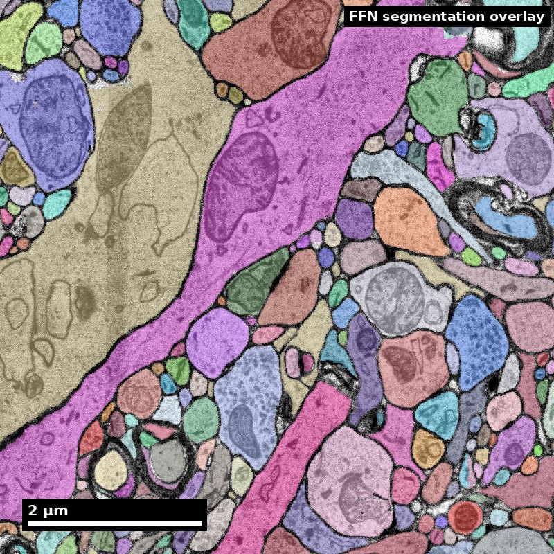
Tools and Methods
Module 8 · EN.585.781 Frontiers in Neuroengineering
Will Gray Roncal · Johns Hopkins University
Part A — From tissue to voxels
Part B — Storage, infrastructure, and what it costs
Part C — Reproducible pipelines
Human cortex · H01
Object segmentation over electron microscopy
H01 release · Lichtman Lab / Harvard & Connectomics at Google
Image: CC BY 4.0 · Shapson-Coe et al. (2024) · doi:10.1126/science.adk4858
Lecture: CC BY-SA 4.0 · neurotrailblazers.org
Figure description and teaching notes
Module 7 asked what a connectome is and what it can support. This module answers a
narrower and more practical question: how does a piece of brain become a dataset that
a hundred people can query, and what makes that dataset trustworthy?
The assignment this week is a real query against a real public volume. Everything in
Part C exists to make that query reproducible six months from now.
Slide 2 of 56
Where we left off
Module 7 established the claim discipline. Module 8 builds the instrument.
Carried forward from Module 7:
- 1 mm³ at 4 × 4 × 40 nm ≈ 1.6 PB raw
- Merges are worse than splits, and understaining causes merges
- Reconstruction scale is always coarser than acquisition scale
- A claim is only as good as the completeness behind it
What Module 8 adds:
Every one of those facts is a consequence of a design decision someone made in the pipeline. This module is those decisions.
The organizing question all module: if this number is wrong, which stage produced the error, and how would I know?
Slide 3 of 56
Learning objectives
By the end of Module 8 you will be able to:
8.1 — Identify the tools and formats used for nanoscale data acquisition, storage, and serving.
8.2 — Trace an artifact in a reconstruction back to the pipeline stage that produced it.
8.3 — Apply the principles of reproducible pipelines to a query against a public connectomics volume.
8.4 — Estimate the capacity, compute, and labor cost of a proposed nanoscale acquisition.
8.3 is the graded artifact: a notebook that returns the same number when someone else runs it next year. That is harder than it sounds, and the reason is Part C.
Slide 4 of 56
Roadmap
Part A — From tissue to voxels The preparation chain, the artifacts each step produces, the imaging tradeoffs, and the QA that catches problems while they are still fixable.
Part B — Storage and infrastructure The eight-stage reference pipeline, chunked multi-resolution arrays, and the capacity and cost model for a petascale volume.
Part C — Reproducible pipelines Why object IDs are not stable, what a materialization version is, and the platform landscape you will actually use.
Standing rule for the module. Every stage exists to solve a specific problem and introduces a characteristic failure. Learn the pairs.
Streams advanced here (Module 7's framing): 2 — throughput and automation, 7 — openness and community, and the infrastructure half of 1 — scale.
Slide 5 of 56
Part A
From tissue to voxels
- The preparation chain and its failure signatures
- Sectioning and imaging families
- Artifact catalog, QA, and acquisition gates
Slide 6 of 56
Where Module 8 sits on the discovery pipeline
The same map from Module 7. This module owns the two middle columns.
   QUESTION        SPECIMEN         IMAGE           RECONSTRUCTION      GRAPH        CLAIM
      |               |               |                   |              |            |
  measurable      fixation        alignment          segmentation    node/edge      null
   endpoint       staining        ingest             proofreading    definition     model
   null model     sectioning      storage            synapses        inclusion      error band
   non-claim      imaging         serving            versioning      boundary       non-claim
      |               |               |                   |              |            |
   Module 7        ===== PART A ===== PART B/C =====    Module 9      Module 9    Module 9
Quality is a ceiling, not a floor. Nothing downstream raises the quality of what acquisition delivered. A segmentation network cannot find a membrane whose metal is not in the tissue.
This is why Part A comes first, and why it is the least glamorous part of the field.
Slide 7 of 56
Projects do not usually die at the algorithm.
They die in the three weeks of chemistry nobody photographed.
A segmentation network cannot find a membrane whose osmium is not in the tissue.
An alignment cannot recover a section that was never collected.
A proofreader cannot resolve an apposition that was never resolvable.
And the failure arrives late. Prep problems surface after acquisition — months and a petabyte later — when the only remaining options are expensive.
The pilot reconstruction (slide 19) exists entirely to move that discovery forward in time.
Slide 8 of 56
Step 1 — Fixation
Arrest ultrastructure within seconds, before autolysis destroys it
Typical protocol. Transcardial perfusion with a buffered aldehyde mix — commonly ~2–2.5% glutaraldehyde plus 2% paraformaldehyde in 0.1 M cacodylate or phosphate buffer, at physiological pH, often with added calcium.
Glutaraldehyde is the workhorse because it is bifunctional and cross-links rapidly. Paraformaldehyde penetrates faster and buys time.
Failure signatures in the final image
- Swollen astrocytic processes, enlarged extracellular space — slow or delayed fixation
- Dark, shrunken, hypercontracted neurons — perfusion pressure or osmolarity
- Blood cells retained in vessels — incomplete perfusion; nearby tissue is likely under-fixed
A trap worth naming. Enlarged extracellular space makes automated segmentation easier — more space between objects. It also distorts every geometric measurement, and it means the tissue you reconstructed is not the tissue that existed in vivo.
Easier to segment is not the same as more correct.
Slide 9 of 56
Step 2 — Contrast generation (staining)
Biological tissue is nearly transparent to electrons. All contrast is heavy metal.
The standard sequence — rOTO
- Osmium tetroxide — binds unsaturated lipids, so it stains membranes. The source of the dark outlines you trace.
- Reduced osmium (with potassium ferrocyanide) — enhances membrane contrast.
- Thiocarbohydrazide (TCH) — a bridging agent that binds bound osmium and offers new sites.
- Second osmium — deposits more metal on the TCH bridges.
- Uranyl acetate, en bloc — general contrast.
- Lead aspartate (Walton) — final enhancement, on the block.
Why rOTO dominates volume EM — two reasons, both structural:
1. Membrane contrast strong enough to image quickly at low dose, which is what makes petascale acquisition finish.
2. The metal load makes the block electrically conductive, which is what makes block-face SEM possible at all without catastrophic charging.
Hua, Laserstein & Helmstaedter 2015 (10.1038/ncomms8923); Mikula & Denk 2015 (10.1038/nmeth.3361) for whole-brain staining.
Slide 10 of 56
Staining failures are the expensive ones
| Failure | How it looks | Downstream cost |
|---|---|---|
| Weak membrane contrast | Thin or interrupted membrane outlines | The dominant cause of automated merge errors — the network cannot find a boundary that is barely there. The single most expensive prep failure. |
| Staining gradient with depth | Block edge well stained, centre pale; reagents did not penetrate | Segmentation quality varies systematically with position — which looks like a biological gradient if you are not careful |
| Precipitate | Small very dark irregular particles, often lead carbonate | False boundaries and false synapse detections; usually tolerable at low density |
The diagnostic question for every defect, all module: which coordinate system does it live in — block position, anatomy, or acquisition time?
Block position → penetration or geometry. Acquisition time → instrument drift or reagent degradation. Anatomy → possibly real biology.
Figure description and teaching notes
The gradient case is worth dwelling on. A depth-dependent staining gradient in a
cortical column runs in the same direction as layer depth. A team that does not check
the coordinate system can publish a "laminar difference in synapse density" that is
entirely a penetration artifact. Ask the room how they would distinguish the two.
Answer: rotate the block relative to the anatomy in a pilot, or check whether the
gradient follows block geometry in a region where the two axes disagree.
Slide 11 of 56
Step 3 — Dehydration and embedding
Water out, resin in — and a tax nobody escapes
Water is replaced by graded ethanol or acetone, then by epoxy resin (Epon/Araldite, LX-112, Durcupan, Spurr's), polymerized to a block that can be cut at tens of nanometers.
The unavoidable cost: dehydration shrinks tissue, typically 5–20% linearly depending on protocol. This is systematic, not random.
Every absolute length, area, and volume measurement in EM connectomics is affected.
What to do about it, practically:
- Report measurements as measured, and state the protocol.
- Prefer ratios and within-volume comparisons to absolute values compared across studies. A ratio between two populations in the same block cancels the shrinkage; an absolute spine-head volume compared to another lab's number does not.
Failure signatures: cracks and tears from too-rapid dehydration or incomplete infiltration; resin too soft or too brittle to section cleanly — which shows up at the next step, not this one.
Slide 12 of 56
Step 4 — Sectioning: two families, two artifact profiles
Serial sectioning (ssTEM / ssSEM) An ultramicrotome with a diamond knife cuts 30–50 nm sections onto grids, tape (ATUM), or a reinforced substrate (GridTape).
Advantage: the block is not consumed by imaging. A section can be re-imaged at higher resolution, and imaging parallelizes across instruments. This is how petascale volumes get acquired in finite time.
Signature artifacts: lost sections, folds, wrinkles, knife chatter (periodic bands perpendicular to the cutting direction), compression along the cutting axis, debris, scratches.
Block-face (SBEM / FIB-SEM) Image the block face, then remove a slice — a diamond knife inside the chamber (SBEM), or an ion beam milling a few nanometers at a time (FIB-SEM).
Advantage: no section handling means no lost sections and dramatically better z-alignment. FIB-SEM's isotropy is the best tracing condition available.
Signature artifacts: the material is destroyed, so nothing can be re-imaged; charging, since the surface is not conductive-coated between cuts; and for FIB-SEM, curtaining — vertical striping from uneven milling.
Denk & Horstmann 2004 (SBF-SEM); Knott 2008 and Xu et al. 2017 (FIB-SEM); Hayworth et al. 2014 (ATUM/WaferMapper), 2015 (hot-knife), 2019 (GCIB-SEM); Phelps et al. 2021 (GridTape).
Slide 13 of 56
Choosing the acquisition modality
| Modality | Voxel | Practical volume | Choose it when | Accept |
|---|---|---|---|---|
| ssTEM / TEMCA | 4 × 4 × 40 nm | Up to ~mm³ | You need a large volume and want the block to survive imaging | Section handling artifacts; heavy alignment work |
| ssSEM + ATUM | 4 × 4 × 30–40 nm | Up to ~mm³ | You want serial sections with robust automated collection onto tape | Tape substrate constraints; re-imaging is possible but slow |
| GridTape TEM | ~4 nm xy | ~10⁵–10⁶ µm³ | You want ssTEM throughput with automated, reel-to-reel section handling | Fixed aperture geometry; specialized infrastructure |
| Multibeam SEM | 4 × 4 × 30–40 nm | ~mm³ in months | Throughput is your binding constraint | Capital cost; a data-handling problem you must solve first |
| SBEM | 10–20 × 10–20 × 25–50 nm | 10⁶–10⁷ µm³ | You want unattended block-face series with no section loss | Destructive; z-resolution limits thin-process tracing |
| FIB-SEM | 4–8 nm isotropic | 10⁵–10⁶ µm³ | Tracing quality dominates and the volume is modest | Slow; hard ceiling on volume per run |
Read the last two columns together. The right question is never "which is best" but "which failure am I willing to own for the next two years?"
Slide 14 of 56
Step 5 — Imaging parameters, and the dose budget
| Parameter | Typical range | Increase it and… | Decrease it and… |
|---|---|---|---|
| Landing energy (SEM) | 1–2 keV | More depth signal, more charging, more beam damage | Better surface specificity, weaker signal |
| Dwell time per pixel | 0.1–2 µs | Better SNR | Faster acquisition, noisier images |
| Beam current | pA–nA | Better SNR at fixed dwell | Less damage and charging |
| Tile overlap | 5–15% | More robust stitching | Less redundant data, faster |
| Section thickness (z) | 30–50 nm | Fewer sections, faster, cheaper | Better z-continuity, more data |
Dose is a budget. SNR improves roughly with the square root of electron dose, and dose = beam current × dwell time. Doubling SNR costs roughly 4× the acquisition time.
This is why "just image it better" is rarely the answer at petascale. The honest trade is usually to accept a noisier image and spend the savings on better segmentation and more proofreading — but never at the cost of membrane contrast, because noise raises splits (recoverable) and faint membranes raise merges (much less so).
Slide 15 of 56
Attacking throughput directly
Multibeam, and what came after
Multibeam SEM (Eberle et al. 2015). 61 or 91 electron beams scanning in parallel, aggregating on the order of a gigapixel per second. This is the technology that moved 1 mm³ from impossible to an eighteen-month project.
FAST-EM array tomography (Kievits & Hoogenboom 2024). A multibeam volume-EM workflow built around optical detection, targeting routine multibeam operation rather than heroic single runs.
SmartEM (2025). Machine-learning-guided acquisition: spend dwell time where the image is hard, not uniformly. The first serious attack on the dose budget itself rather than on the beam count.
Read these as three different moves on the same constraint.
Multibeam parallelizes the instrument. FAST-EM industrializes the workflow. SmartEM makes the dose allocation adaptive.
Only the third changes the square-root relationship that governs everything else — and it is the one to watch.
Slide 16 of 56
Buying volume back for FIB-SEM
Two engineering moves that change the ceiling rather than the tradeoff
Hot-knife partitioning (Hayworth et al. 2015). Cut the block into thick slabs with an ultrastructurally smooth interface, image each slab by FIB-SEM independently, then stitch the volumes back together.
FIB-SEM's volume limit is per-run. Partitioning turns one impossible run into many feasible ones, at the cost of a small number of well-characterized interfaces.
GCIB-SEM (Hayworth et al. 2019). A gas cluster ion beam removes material more gently and over a wider area than a focused ion beam, reaching ~10 nm isotropic on much larger tissue faces.
Why this pattern is worth naming.
Most progress in this field is not a better microscope. It is someone noticing that a hard constraint is actually a per-run constraint, and finding a way to partition the problem.
Hot-knife does it for volume. Multibeam does it for throughput. SmartEM does it for dose. Community proofreading does it for labor.
When you meet a ceiling, ask what it is per.
Slide 17 of 56
Alternative routes: when the EM chain is not the only chain
Expansion microscopy. Physically swell the specimen in a hydrogel so that diffraction-limited optics resolve ~25–70 nm effective features. Buys molecular identity alongside near-EM geometry — the one thing standard EM cannot give.
Costs: expansion distortion that must be characterized, and dense reconstruction at scale is not yet routine.
LICONN (Tavakoli et al. 2025). Light-microscopy-based connectomic reconstruction of mammalian brain tissue — the first demonstrated LM route to dense, synapse-level reconstruction.
Why this belongs in a tools module rather than a news slide.
If an LM route scales, several Part B line items change at once: no ultramicrotome, no section loss, protein labels available in the same specimen, and a very different storage and staining economics.
It does not make EM obsolete — resolution, validation history, and dense-neuropil performance still favor EM today. But the cost argument from Module 7 is the thing under pressure, and that is worth tracking deliberately.
Tavakoli et al. 2025, 10.1038/s41586-025-08985-1.
Slide 18 of 56
Worked example: how long does acquisition take?
A volume is 800 µm × 800 µm × 800 µm at 4 × 4 × 40 nm. Your instrument sustains 0.2 gigapixels per second including overheads. How long?
voxels_xy per section = (800,000 / 4)^2 = 200,000^2   = 4.0 x 10^10 px
sections              =  800,000 / 40                 = 20,000
total pixels          = 4.0e10 x 2.0e4                = 8.0 x 10^14 px

time = 8.0e14 / 2.0e8 px/s = 4.0 x 10^6 s             ~= 46 days continuous
Then multiply by your real duty cycle. At 60% uptime this is ~77 days — and that counts only imaging. Not sectioning. Not QA. Not re-imaging failed sections.
When someone says a 1 mm³ volume takes "about a year", this is the arithmetic behind it. You now have both halves of the sizing calculation: Module 7 gave you petabytes, this gives you months.
Slide 19 of 56
The artifact catalog
| Artifact | Recognize it by | Root cause | Downstream effect | Cost class |
|---|---|---|---|---|
| Lost section | A z-gap; structures discontinuous across one z index, volume-wide | Section lost in collection | Every process crossing that z must be bridged by inference | Data loss |
| Fold | Dark band with duplicated/compressed tissue | Section wrinkled on collection | Tissue in the fold unusable; segmentation splits along it | Data loss |
| Tear / crack | Sharp-edged gap, often following a vessel | Dehydration or sectioning stress | Local loss; false boundaries at edges | Data loss |
| Knife chatter | Periodic bands, fixed spacing, ⟂ cutting direction | Knife or block vibration | False boundaries; raises split rate | Labor |
| Compression | Section short along the cutting axis | Knife compresses the section | Systematic geometric distortion | Labor + measurement bias |
| Charging | Bright streaks trailing the scan direction | Non-conductive surface | Model confidence collapses locally; splits | Labor |
| Curtaining (FIB-SEM) | Vertical stripes ∥ milling direction | Uneven milling rate | Degrades boundary detection | Labor |
| Weak membrane contrast | Faint or interrupted membranes | Understaining | Merge errors — the expensive kind | Labor, high |
| Precipitate | Small very dark irregular particles | Staining chemistry | False synapse detections | Labor, low |
| Beam damage | Bubbling, mass loss, progressive contrast change | Excess dose | Worsens with re-imaging | Data loss if severe |
| Misalignment / drift | Structures shift between adjacent sections | Stitching or registration failure | False branch points; synapse mislocalization | Labor, correctable |
| Seam visibility | Intensity step at tile boundaries | Stitching / illumination correction | Boundary artifacts on a regular grid | Labor, correctable |
Slide 20 of 56
Two cost classes, and why the distinction is the point
Labor artifact → your reconstruction will be correct eventually, after paying in proofreading hours or better algorithms.
Data loss artifact → some biological question is unanswerable in that region, permanently.
A QA report that gives one quality score conceals exactly the distinction the project needs. Report them separately.
Rank for triage on a 20,000-section volume: (a) 4 lost sections scattered, (b) 4 consecutive lost sections, (c) charging on 15% of sections, (d) 10% weaker membrane contrast throughout.
(b) > (d) > (c) > (a).
(b) = a 160 nm gap. Most thin neurites cannot be bridged; the volume is effectively two independently reconstructable halves. (d) raises the merge rate everywhere, invisibly, and cannot be fixed by re-imaging — the metal is not in the tissue. (c) is bounded and mostly raises splits. (a) is normal operating loss. Log it; do not panic.
Transferable lesson: distribution matters more than count. Four scattered losses and four consecutive losses have the same headline number and completely different consequences. Never report an artifact rate without its spatial distribution.
Slide 21 of 56
Acquisition QA that actually catches problems
The non-negotiable rule
Run a pilot reconstruction before full acquisition. Take ~100 × 100 × 100 µm through the entire pipeline — align, segment, skeletonize, and have a human proofread a handful of neurons. Measure the error rate.
This costs perhaps 1–2% of the project, and it is the only way to discover that your staining protocol produces a merge rate the segmentation cannot handle while you can still change the staining protocol.
Metrics to log continuously — per section and per tile, not just per volume:
- Intensity distribution — mean, sd, 1st/99th percentiles. Drift is the earliest warning.
- Membrane contrast-to-noise. Practical proxy: (membrane trough − cytoplasm median) ÷ noise σ, sampled across many profiles. Track the trend, not the absolute value.
- Focus / sharpness proxy — high-frequency energy fraction of the power spectrum.
- Section thickness, empirically. Cross-check nominal against a traced mitochondrion or myelinated axon. Nominal ≠ actual, and z-step error propagates into every length measurement.
- Stitching and alignment residuals — as a distribution, with the maximum.
- Defect masks — machine-readable, stored with the volume, surfaced in the viewer.
Slide 22 of 56
Gates: define what stops acquisition, in advance
| Gate | Example threshold | Action if breached |
|---|---|---|
| Consecutive lost sections | > 2 | Stop. Investigate collection before continuing |
| Cumulative lost-section rate | > 1% | Review handling protocol |
| Membrane CNR drop vs baseline | > 20% | Stop. Check staining batch and beam conditions |
| Fold area fraction per section | > 5% | Flag section; re-cut if the block allows |
| Alignment residual, 99th percentile | > 1 voxel at native xy | Re-run alignment before ingesting |
| Pilot segmentation merge rate | Above what your proofreading budget absorbs | Do not scale. Revisit prep |
The specific numbers are yours to set — they depend on your endpoint and your budget. What is not optional is setting them before you start, in writing.
A threshold chosen after seeing the data is not a threshold.
Slide 23 of 56
Part A checkpoint — provenance, and why per-tile timestamps matter
The minimum machine-readable record, for every derived product:
- Specimen — species, strain, age, sex, region, fixation protocol and timings
- Staining — protocol, reagent lots, incubation times, temperatures
- Embedding — resin, polymerization schedule
- Sectioning — nominal thickness, knife, substrate, operator, session
- Imaging — instrument and serial number, landing energy, beam current, dwell time, detector, tile size and overlap, pixel size, acquisition timestamp per tile
- Processing — every transform applied, with parameters and software version
Why the tile-level timestamp earns its place. When you later find a quality anomaly, the first diagnostic question is always: does this defect follow block position, anatomy, or acquisition time?
Time-correlated → instrument drift or reagent degradation. Position-correlated → penetration or geometry.
Without per-tile timestamps you cannot ask the question at all.
Slide 24 of 56
Part A checkpoint — four things to stop believing
"Better images are always worth it." Dose is a budget and SNR goes as its square root. Doubling SNR costs ~4× the time. Spend it on membrane contrast, not on general prettiness.
"Open-looking neuropil is good data." It segments more easily and it means the fixation distorted the tissue. Easier is not more correct.
"An artifact rate summarizes an artifact." Four scattered lost sections and four consecutive ones have the same rate and entirely different consequences. Distribution beats count.
"We will assess quality when acquisition finishes." Then you will assess it having spent the budget. The pilot reconstruction is 1–2% of the project and it is the only stage where the answer can still change the protocol.
Break. Part B: what happens to those voxels once they exist.
Slide 25 of 56
Part B
Storage, infrastructure, and what it costs
- The eight-stage reference pipeline
- Chunked multi-resolution arrays, and why chunk shape is a real decision
- Capacity, compute, and the cost that dominates all of them
Slide 26 of 56
The reference pipeline: eight stages, eight artifacts
| Stage | Input | Output artifact |
|---|---|---|
| 1 — Ingest | Raw tiles + acquisition metadata | Immutable, checksummed archive + validated tile manifest |
| 2 — Stitch and align | Tiles | Coherent 3D volume + the transform stack that produced it |
| 3 — Boundary/affinity prediction | Aligned image | Per-voxel affinity or boundary map, same size as the input |
| 4 — Supervoxel generation | Affinities | Supervoxels — deliberately over-segmented, immutable fragments |
| 5 — Agglomeration | Supervoxels + affinities | The segmentation: an assignment of supervoxels to objects |
| 6 — Derived geometry | Segmentation | Meshes (multi-LOD), skeletons, per-object statistics |
| 7 — Synapse detection | Aligned image (+ segmentation) | Synapse table: coordinates, pre/post IDs, confidence, size |
| 8 — Annotation and serving | Everything above | Interactive viewing, proofreading, queries, versioned tables |
Learn what each artifact is, because that is what you will debug. "The segmentation is wrong" is not actionable. "Stage 3 has block-boundary seams on a 512³ grid" is.
Slide 27 of 56
What "write-once" actually means in practice
An ingest checklist, because this is the one stage you cannot redo
-
Checksum every tile on arrival, and store the checksums separately from the tiles. A silently corrupted tile discovered two years later is indistinguishable from a biological oddity.
-
Validate the manifest against the tiles. Every tile the microscope claims to have written exists, has the expected dimensions, and carries its metadata.
-
Join metadata to tiles at ingest, not later. Position, timestamp, beam conditions, session, operator. Metadata that arrives as a spreadsheet a month later will not be joined correctly, ever.
-
Write to immutable storage with object versioning and a lifecycle policy that moves it to cold tiers once validated.
-
Record the ingest itself — who, when, from which instrument, with which tool version.
The test of an ingest stage: could you re-run the entire downstream pipeline from scratch, five years from now, with nobody from the original team available? If not, the archive is not an archive; it is a copy.
Slide 28 of 56
Stage 1–2 — Ingest, stitching, and alignment
Ingest. The archive is write-once. Nothing downstream ever modifies it. If a later stage is wrong, you re-run from here.
Treat the raw archive as the only irreplaceable asset in the project — everything else is recomputable, expensively.
Common failure: metadata that is not machine-readable, so tile position, timestamp, and acquisition parameters cannot be joined to defects found later.
Stitching (within a section) places tiles using their overlap. Mostly rigid or affine per tile.
Alignment (across sections) registers section n to n−1. Hard, because sections deform non-rigidly and errors accumulate:
A 0.1-voxel-per-section bias over 20,000 sections is a 2,000-voxel drift.
Modern pipelines use coarse-to-fine elastic registration with a global relaxation step that distributes residual error across the whole stack rather than letting it accumulate in one direction.
What you must retain: the transforms, versioned. Any coordinate in aligned space is meaningless without knowing which alignment version produced it. When alignment is revised, every stored annotation coordinate must be re-mapped — which is why alignment revisions are rare and carefully planned.
Saalfeld et al. 2012 (10.1038/nmeth.2072, elastic alignment); SOFIMA (Google, flow-based alignment).
Slide 29 of 56
Stage 3–5 — Affinities, supervoxels, agglomeration
Stage 3 — affinity prediction. A dense convolutional network applied over petavoxels. The most compute-intensive stage, embarrassingly parallel over blocks — with the caveat that blocks must overlap, because the network needs context beyond the region it predicts.
Common failure: block-boundary seams, visible later as a regular grid of segmentation errors. Detect it by asking whether the error distribution matches your block grid. (Part A's coordinate-system question again.)
Stage 4 — supervoxels. Watershed at a threshold that guarantees over-segmentation: a supervoxel may be a piece of a neurite, but it should almost never span two neurites.
The pipeline accepts many splits in order to avoid merges — because merges are the expensive error. This single decision propagates to every downstream design choice in the module.
Stage 5 — agglomeration. Mean-affinity, learned agglomeration with local shape descriptors, or flood-filling networks growing objects from seeds. Architecturally, the output is a grouping of immutable atoms, not a new voxel labeling.
Slide 30 of 56
Stage 6–7 — Geometry and synapses
Derived geometry. Meshes for 3D viewing (multi-LOD), skeletons for morphometry and path distance, per-object statistics.
These are regenerated when the segmentation changes, which is constantly. Design them as cheap, incremental, and per-object. A geometry pipeline that must run volume-wide to reflect one proofreading edit is a pipeline that will not run.
Synapse detection. A separate detection problem with its own network. Output: a table of coordinates, pre/post identity, confidence, cleft size.
Store partner identity as supervoxel IDs, not object IDs.
Supervoxel IDs are immutable, so when proofreading changes which neuron an object is, the synapse assignment follows automatically.
Storing object IDs means rewriting the synapse table on every edit — a design mistake that is easy to make and painful to undo.
SynEM (Staffler et al. 2017, 10.7554/eLife.26414); SyConn (Dorkenwald et al. 2017, 10.1038/nmeth.4206); Synful partner prediction (Buhmann et al. 2021, 10.1038/s41592-021-01183-7).
Slide 31 of 56
How pipeline errors present downstream
Each defect has a signature. Learn to read backwards from the symptom.
| What you see in the reconstruction | Most likely stage | Why |
|---|---|---|
| Segmentation errors on a regular 3D grid | Stage 3 — affinity prediction | Insufficient block overlap; the network lacked context at block edges |
| False branch points, structures jumping between adjacent z | Stage 2 — alignment | Section-to-section registration failure; the branch is two objects misregistered |
| Errors concentrated at tile seams on a 2D grid | Stage 2 — stitching | Illumination correction or seam blending failure |
| Objects truncated at one z plane, volume-wide | Acquisition | Lost section — a data-loss artifact, not a segmentation problem |
| Merge rate rising smoothly with depth into the block | Staining | Penetration gradient; follows block geometry |
| Merge rate rising with acquisition order | Imaging | Beam or detector drift; follows time |
| Synapse counts that changed since last month, same cell | Stage 8 / proofreading | You queried latest. See Part C. |
The move is always the same: identify which coordinate system the defect lives in — block position, anatomy, acquisition time, or processing grid — and that identifies the stage.
Slide 32 of 56
Serving: the precomputed contract
Why a browser can fly through a petabyte
The contract Neuroglancer relies on is simple and worth understanding, because everything else in the ecosystem is built to satisfy it:
- data lives at predictable URLs derived from (scale, chunk coordinates)
- an info JSON declares voxel size, extents, data type, and the available scales
- the client requests only the chunks in view, at the coarsest adequate scale
- there is no server-side computation — an object store is enough
The consequence is the field's quiet superpower. Because serving is just static objects, anyone can host a volume, and any client that speaks the format can read it. Neuroglancer, CloudVolume, and a dozen analysis tools interoperate without negotiating anything.
Compare this to a database that must be running for the data to exist.
Precomputed format spec: github.com/google/neuroglancer. Zarr / OME-Zarr and N5 make the same architectural bet with different conventions.
Slide 33 of 56
Storage: chunked, multi-resolution arrays
The Neuroglancer precomputed format, N5, Zarr / OME-Zarr, and relatives
Chunks. The volume is divided into blocks — commonly 64³ to 512³ voxels — stored as individual objects. You fetch only the chunks you need. This is the whole reason interactive viewing of a petabyte is possible.
Resolution pyramid. Progressively downsampled copies. Zooming out fetches a coarse level instead of a million fine chunks. Costs about 30–50% extra storage.
Sharding. Millions of tiny objects are slow and expensive in object stores, so chunks are bundled into larger shard files with an index. A pure cost/latency optimization that matters enormously at petascale.
Compression. Lossy (JPEG) for image data, where a little compression noise is acceptable. Lossless and label-aware for label data — where a single flipped bit changes an object's identity.
Figure description and teaching notes
The compression asymmetry is worth pausing on. Students often assume label data
compresses better because it is "simpler". It does — but the tolerance for error is
zero, which is why compressed-segmentation encodings exist as a separate format family
rather than reusing image codecs.
Slide 34 of 56
Chunk shape is an access-pattern decision
And the three consumers want opposite things
| Consumer | Access pattern | Wants |
|---|---|---|
| Proofreader in a viewer | Scrolls through z at one xy location, then pans | Chunks elongated in z, or at least isotropic in index space |
| Analysis job | Reads a whole neuron's bounding box, or a whole section | Large chunks, sequential layout |
| Synapse query | Random access to scattered small regions | Small chunks, good spatial index |
You cannot optimize for all three with one layout.
Production systems store multiple representations — the image pyramid for viewing, the segmentation graph for editing, and materialized tables for analysis — precisely so each consumer gets a layout suited to it.
When someone asks "why is this stored three times?" — that is the answer.
Slide 35 of 56
Capacity, worked, for 1 mm³ at 4 × 4 × 40 nm
| Item | Estimate | Notes |
|---|---|---|
| Raw archive | ~1.5 PB | Written once, read rarely → cold storage |
| Aligned pyramid | ~2 PB | Base + 30–50% pyramid; hot |
| Affinity / boundary maps | ~1.5 PB | Often transient — delete after supervoxel generation |
| Supervoxels + segmentation | 0.2–0.8 PB | Label-aware compression helps a lot |
| Meshes (all LODs) | 1–10 TB | Regenerated on edit |
| Skeletons | 10–100 GB | Cheap — archive them |
| Synapse table | 50–200 GB | ~5 × 10⁸ rows; the hottest analytical table |
| Edit history | Grows monotonically | Must be curated, never deleted |
The operational lesson. The raw volume is written once and read rarely. The synapse table and the segmentation are read constantly, by many people, with latency expectations in milliseconds.
Budget for query load, not just capacity. A petabyte in cold object storage is cheap. A 200 GB table answering 50 concurrent interactive queries is the part that needs engineering.
Slide 36 of 56
Compute cost, and the one that actually dominates
GPU cost, order of magnitude. Suppose a segmentation network processes ~10⁷ voxels/second/GPU end-to-end including I/O. For 1.5 × 10¹⁵ voxels:
1.5e15 / 1e7 = 1.5e8 GPU-seconds
             ~= 1,736 GPU-days
On 500 GPUs, roughly 3.5 days of wall clock — and you will run it more than once, because the first model version is never the last.
Budget 3–5 full inference passes over the project lifetime.
But the dominant cost is none of the above. It is proofreading labor.
At even a few hours of skilled human attention per fully-proofread neuron, a study needing 1,000 complete neurons is thousands of person-hours.
Compute and storage are line items you can negotiate with a cloud vendor. Proofreading is a hiring, training, retention, and quality-management problem — and it is why Module 9 Part A spends its time on triage rather than on algorithms.
Slide 37 of 56
Cost traps specific to this domain
-
Egress. Moving a petabyte out of a cloud region can cost more than storing it for a year. Co-locate compute with data; give collaborators compute next to the data rather than copies of it.
-
Small-object overhead. Billions of unsharded chunks incur per-request charges and listing costs that can exceed storage costs. Shard.
-
Forgotten intermediates. Affinity maps are the size of the raw data. Delete them after supervoxel generation, or set a lifecycle policy — but only once you are confident you will not need to re-agglomerate.
-
Idle hot storage. Move the raw archive to cold tiers immediately after ingest validation.
Part B checkpoint. Take your Module 7 study brief and put a number on it: raw petabytes, months of imaging, GPU-days, and — the one that decides feasibility — proofreading person-hours. If any of the four is unknown to within an order of magnitude, the brief is not yet a plan.
Slide 38 of 56
Annotation tables and spatial queries
The layer where analysis actually happens
What lives here. Synapses, cell-type calls, manual annotations, proofreading status, nucleus detections, per-cell statistics — each a table keyed to the segmentation.
Two query shapes dominate, and they need different indexes:
Relational. "Give me every synapse where the presynaptic object is in this list of root IDs." Wants an index on object identity, and a join to the current segmentation state.
Spatial. "Give me every synapse in this bounding box." Wants a spatial index — and at 5 × 10⁸ rows the difference between having one and not is the difference between milliseconds and minutes.
The join to segmentation state is where versions bite. A synapse table row stores supervoxel IDs. Turning those into "which neuron?" requires the ChunkedGraph as of a timestamp. That lookup is exactly what a materialization freezes — and why Part C is the next slide and not an appendix.
Slide 39 of 56
Part C
Reproducible pipelines
- Why object IDs are not stable
- Materialization versions, and the number-one silent failure
- The platform landscape, and this week's assignment
Slide 40 of 56
The number-one reproducibility failure in connectomics analysis
is silent.
Your code runs fine. It just answers a different question than it did last week.
Why? Because object IDs are not stable.
Slide 41 of 56
The problem, and the design that solves it
The naive design. Store the segmentation as a labeled volume. Then a proofreader merges two neurons and you rewrite… potentially gigabytes of voxels.
With hundreds of proofreaders editing concurrently, this is unworkable.
The ChunkedGraph solution. Store supervoxels once, immutably. Represent the segmentation as a graph whose nodes are supervoxels and whose edges say "these are the same object." An object is a connected component of that graph.
- A merge is adding an edge. Microseconds, not gigabytes.
- A split is removing edges — a minimum cut separating two user-specified points.
- The graph is hierarchical and chunked, so component queries over millions of supervoxels stay fast.
- Every edit is an entry in an append-only log, with author, timestamp, operation. Nothing is destroyed; any past state is recoverable.
- Concurrent editing works, because edits are small graph operations reconciled independently.
CAVE / PyChunkedGraph (Dorkenwald et al., 10.1038/s41592-024-02426-z); DVID (Katz & Plaza 2019); CATMAID (Saalfeld et al. 2009) solved the related problem for skeleton tracing.
Slide 42 of 56
The consequence for you, the analyst
In a ChunkedGraph system, merges and splits can change a neuron's root ID. A root ID identifies a reconstructed object at a particular segmentation state.
An object ID in your notebook, your paper, or your figure caption is meaningless without a timestamp or version.
Materialization is the fix. The system periodically produces a frozen snapshot in which every annotation — synapses, cell-type labels, manual annotations — has been joined to the segmentation state at a specific timestamp, and written into queryable tables.
- Analyses run against a materialization version, e.g. version 943.
- The version number is a first-class part of your methods section, exactly like a software version or a genome build.
- Re-running on a later version may give different numbers. Compare the segmentation state, table and query before attributing a change to proofreading.
Slide 43 of 56
Worked example: which version produced this number?
Hypothetical situation. A figure reports 1,412 input synapses. A rerun returns 1,530 for an ID the lineage viewer links to the same cell. A reviewer asks which number is right.
Step 1 — look for the pin. Inspect the materialization version, timestamp, table, object mapping and query. An unpinned run leaves the inputs uncertain.
Step 2 — compare the evidence. Check archived results and query logs. Version changes, filtering differences or object remapping could change the count. The discrepancy alone does not identify the cause.
Step 3 — reproduce before interpreting. Run the recorded query against the recorded inputs. If provenance is missing, label the earlier result unreproduced rather than declaring both counts correct.
Step 4 — retain the record. Archive the inputs, code, environment and outputs. A version pin or checksum cannot recover a file that nobody retained.
Slide 44 of 56
The reproducibility header
Six lines at the top of every notebook. Non-negotiable.
# --- reproducibility header -------------------------------------------
DATASET        = "minnie65_public"      # dataset name, not "the volume"
MAT_VERSION    = 943                    # pinned; never "latest"
QUERY_DATE     = "2026-03-14"           # when this ran
CODE_REV       = "a3f9c21"              # git commit of THIS notebook
CLIENT_VERSION = "caveclient 5.21.0"    # and its dependencies
SEED           = 20260314               # any stochastic step
# ----------------------------------------------------------------------
The rule. Every figure records the materialization version, the query code, and the date. Every paper states the version.
If your collaborator cannot reproduce your number, the first question is always "which version?" — and it should be answerable in one second, from the figure.
Figure description and teaching notes
For the 90-minute teaching session, use the offline Tools and Methods worksheet
and query linked from /teaching/lectures/connectomics-02-tools-and-methods/.
The example below illustrates fields, not a verified current public-data query.
Ask learners to supply actual values from their run. Do not copy example versions
or a fabricated code revision. Record coordinate frame and units for spatial queries.
Make them physically add this to the assignment notebook. It is the single highest-value
habit in the module, it takes ninety seconds, and essentially nobody does it until they
have been burned once. The assignment rubric awards points for it explicitly.
Slide 45 of 56
The other four reproducibility requirements
Every stage output records: input artifact IDs, code revision (commit hash), the full parameter set, model artifact hash and framework version, container image digest, random seeds, and wall-clock/resource usage.
Idempotency. Re-running a stage on the same inputs with the same parameters produces the same output. This sounds trivial and is not — GPU non-determinism, unpinned dependencies, and unseeded randomness all break it. Pin them explicitly and test that a re-run matches.
Region-scoped invalidation. When a region is re-processed, only downstream artifacts for that region are invalidated. A pipeline whose only recovery option is "re-run everything" cannot fix a local defect at petascale — so this is a structural requirement, not a nicety.
Release candidates. Segmentation is versioned and released like software: produce a candidate, compute quality metrics (Module 9), review, then promote or reject. Analyses cite the release.
Slide 46 of 56
Environments: pinning, containers, and the honest re-run test
Pin the whole stack, not the top of it.
- Exact package versions — a lockfile, not a range
- The container image digest, not a
:latesttag - CUDA/driver versions where GPU results are involved
- Random seeds for every stochastic step
Then test it. Run the pipeline twice in fresh environments and diff the outputs. Most pipelines fail this the first time, and the failure is always informative.
Known idempotency breakers, in order of how often they bite:
- Unpinned transitive dependencies — a patch release changes a default
- Unseeded randomness in augmentation, sampling, or initialization
- GPU non-determinism — reduction order in cuDNN kernels
- Filesystem ordering —
globreturning files in a different order - Wall-clock or hostname leaking into an output path or a seed
Items 1 and 4 are free to fix. Item 3 may cost throughput to fix, and that is a decision to make deliberately and record, not to discover.
Slide 47 of 56
Sharing: FAIR, licensing, and what "public" actually means
Findable. A persistent identifier and rich metadata — not a lab web page that moves when a postdoc graduates.
Accessible. An open protocol. Precomputed-over-HTTP satisfies this almost by accident, which is part of why it won.
Interoperable. Standard formats and vocabularies, so a second tool can read your volume without a bespoke adapter.
Reusable. A clear license, and provenance detailed enough for someone to judge fitness for their purpose — not just yours.
"Publicly available" is not one thing. Ask which of these a dataset actually offers:
- viewable in a browser, but not downloadable
- downloadable, but no license stated
- licensed, but no provenance
- everything above, but egress costs are yours
The fourth is the common case at petascale, and it is why co-located compute matters more than "open data" as a slogan.
Human tissue adds a layer. Consent frameworks, de-identification, and IRB conditions travel with the data. State them in the dataset record, not in an email.
Slide 48 of 56
The platform landscape
| Platform | What it is | Reach for it when |
|---|---|---|
| Neuroglancer | Browser-based viewer for precomputed volumes | You want to look at any volume. The universal client. |
| CloudVolume / Igneous | Python library for reading/writing precomputed data; distributed processing | You want programmatic access to voxels, meshes, skeletons |
| BossDB | Community archive and API across many datasets | You need MICrONS, H01, Kasthuri, Witvliet, zebrafish from one interface |
| CAVE / PyChunkedGraph | Versioned proofreading + annotation backend | You are querying MICrONS or FlyWire with versions |
| neuPrint | Neo4j-backed graph service over released connectomes | You want a connectivity graph query and no infrastructure work |
| DVID | Distributed versioned image-oriented dataservice | Janelia-lineage pipelines |
| webKnossos | Browser-based annotation and proofreading | You need to annotate, in a browser, with a team |
| CATMAID | Collaborative skeleton-tracing over massive image data | Fly larva and FAFB-lineage tracing |
BossDB (10.1038/s41592-018-0181-1); neuPrint (10.3389/fninf.2022.896292); CAVE (10.1038/s41592-024-02426-z); DVID (10.3389/fncir.2019.00005); webKnossos (10.1038/nmeth.4331); VAST (10.3389/fncir.2018.00088).
Slide 49 of 56
Choosing a platform for the assignment
Start with neuPrint if you want connectivity fast. The connectome is frozen, the graph is served, and there is no version problem to reason about — which is a feature for a first query and a limitation later.
Use CAVE / caveclient if you want MICrONS or FlyWire with the versioning machinery. This is the realistic case and the one the assignment rewards.
Use CloudVolume / BossDB if your question needs voxels, meshes, or skeletons rather than a graph.
A good assignment query is small and specific.
"For MICrONS materialization v943, what is the distribution of synapse counts per connection among proofread L2/3 pyramidal cells?"
Pinned version. Named population. A distribution, not a single number. Runs in minutes. Reproducible by a stranger.
Slide 50 of 56
What has to change for a whole mouse brain
500× is an engineering program, not a microscope purchase
| Bottleneck | Where it is today | What the 500× demands |
|---|---|---|
| Sectioning reliability | Lost-section rates tolerable at 20,000 sections | Millions of sections; the same rate becomes catastrophic |
| Acquisition throughput | ~1 Gpx/s with multibeam | Adaptive dose (SmartEM), more parallel instruments, industrialized workflow |
| Alignment robustness | Human intervention at hard regions | Must be unattended, or the human cost scales with the volume |
| Segmentation accuracy | Good enough that proofreading is affordable at mm³ | Error rates must fall faster than volume rises |
| Proofreading labor | The dominant cost already | Automated error detection, better triage, community proofreading |
| Storage economics | ~2 PB hot per mm³ | ~800 PB; egress and query load become the design constraint |
Note which row is bold. Every other row is a research problem with an obvious line of attack. Proofreading is the one where the answer is not yet in view — which is exactly why Module 9 opens there.
Slide 51 of 56
Part C checkpoint — a five-minute reproducibility audit
Run this on any connectomics figure, including your own
| Ask | Red flag |
|---|---|
| Which dataset, named precisely? | "The MICrONS data" — which release? |
| Which materialization version? | Absent, or latest |
| Which code, at which revision? | "Available on request" |
| What inclusion criteria produced this population? | n stated, criteria not |
| What synapse threshold built the graph? | Unstated — see Module 9 |
| What error rates, and how do they propagate to this number? | "The data were proofread" |
| Could a stranger re-run it? | Only the first author has the environment |
Do this to your own assignment notebook before submitting it. Every row you cannot answer is a point the rubric will find, and — more usefully — a question a reviewer would have asked eighteen months from now, when you no longer remember.
Slide 52 of 56
Module 8 assignment
Five short-answer questions plus a reproducible query. Due before Module 9.
Short answer. Acquisition-time arithmetic; an artifact triage ranking with justification; a capacity estimate; a chunk-shape choice for a stated access pattern; diagnosing a defect by its coordinate system.
The reproducible query (graded artifact). A notebook that:
| Requirement | Why it is graded |
|---|---|
| Carries the six-line reproducibility header | The version is the whole point |
Pins a materialization version — never latest |
Otherwise the result is not a result |
| Answers one specific question about a named population | Scope discipline |
| Reports n, and what was excluded and why | Inclusion criteria are the least-reported decision |
| States one limitation the data cannot address | The Module 7 non-claim, carried forward |
| Runs end to end from a clean environment | If it only runs on your laptop, it does not run |
Slide 53 of 56
Discussion forum and journal club
Discussion prompt 1 — the artifact you would fear most. Pick one artifact from the catalog. Argue for where it belongs in the labor/data-loss split, and describe the QA metric that would catch it earliest. Disagree with a classmate who ranked it differently.
Discussion prompt 2 — the version problem in your field. Every field has a version problem: genome builds, atlas versions, model checkpoints. Describe one from your own area, and what the community did (or failed to do) about it.
Journal club — a methods paper this week. Choose one:
- Januszewski et al. 2018 — flood-filling networks
- Dorkenwald et al. 2025 — CAVE
- Kievits & Hoogenboom 2024 — FAST-EM
- SmartEM 2025 — ML-guided acquisition
- Tavakoli et al. 2025 — LICONN
Present the problem the method solves, the cost it pays, and the claim you think it does not support.
Slide 54 of 56
What to bring to Module 9
Module 9 turns voxels into claims. Segmentation and its error metrics, proofreading triage, graph construction, null models, motifs, and what connectomics and machine learning actually give each other.
Come with:
- your reproducible query, run and working
- the merge/split asymmetry, which becomes quantitative
- your Module 7 study brief — Module 9's lab makes it a real analysis plan
The one idea to carry forward.
Every number in connectomics is produced by a versioned pipeline whose stages each have a characteristic failure.
Reproducibility is not paperwork. It is the only thing that lets you say which number you are defending.
Slide 55 of 56
References and sources
Preparation and staining. Hua, Laserstein & Helmstaedter 2015 (10.1038/ncomms8923, rOTO en-bloc); Mikula & Denk 2015 (10.1038/nmeth.3361, whole-brain staining); Pallotto et al. 2015 (10.7554/eLife.08206, ECS-preserving fixation).
Sectioning and acquisition. Denk & Horstmann 2004 (10.1371/journal.pbio.0020329); Knott et al. 2008 (10.1523/JNEUROSCI.3189-07.2008); Bock et al. 2011 (10.1038/nature09802, TEMCA); Hayworth et al. 2014 (10.3389/fncir.2014.00068, ATUM + WaferMapper), 2015 (10.1038/nmeth.3292, hot-knife), 2019 (10.1038/s41592-019-0641-2, GCIB-SEM); Eberle et al. 2015 (10.1111/jmi.12224, multibeam); Xu et al. 2017 (10.7554/eLife.25916); Phelps et al. 2021 (10.1016/j.cell.2020.12.013, GridTape); Kievits & Hoogenboom 2024 (10.1515/mim-2024-0005, FAST-EM); SmartEM 2025 (10.1038/s41592-025-02929-3).
Alignment, segmentation, synapses. Saalfeld et al. 2012 (10.1038/nmeth.2072); SOFIMA (github.com/google-research/sofima); Januszewski et al. 2018 (10.1038/s41592-018-0049-4, flood-filling); Berning et al. 2015 (10.1016/j.neuron.2015.09.003, SegEM); Funke et al. 2019 (10.1109/TPAMI.2018.2835450); Staffler et al. 2017 (10.7554/eLife.26414, SynEM); Dorkenwald et al. 2017 (10.1038/nmeth.4206, SyConn); Buhmann et al. 2021 (10.1038/s41592-021-01183-7, Synful).
Infrastructure. BossDB (10.1038/s41592-018-0181-1); neuPrint (10.3389/fninf.2022.896292); CAVE (10.1038/s41592-024-02426-z); DVID (10.3389/fncir.2019.00005); webKnossos (10.1038/nmeth.4331); CATMAID (10.1093/bioinformatics/btp266); VAST (10.3389/fncir.2018.00088); CloudVolume (github.com/seung-lab/cloud-volume); Neuroglancer (github.com/google/neuroglancer).
Course material. NeuroTrailblazers technical training Units 03, 04.
https://neurotrailblazers.org
Slide 56 of 56
Use, adapt, and credit
These slides are openly licensed for community use
Licence: CC BY-SA 4.0
Creative Commons Attribution-ShareAlike 4.0 International.
https://creativecommons.org/licenses/by-sa/4.0/
You may teach from these slides anywhere, including commercially; copy and redistribute them in any medium; and re-cut, shorten, translate, restyle, or merge them into your own material — and distribute the result. No permission needed.
Two conditions. Attribution — credit the original, link the licence, and say if you changed anything. ShareAlike — distribute your adapted version under this same licence, so it stays as open as what it came from.
How to credit
Gray Roncal, W. (2026). Nanoscale Connectomics: Tools and Methods (EN.585.781 Frontiers in Neuroengineering, Module 8). NeuroTrailblazers. CC BY-SA 4.0. neurotrailblazers.org/teaching/lectures/
For an adaptation, prefix with "Adapted from" and note what you changed.
Editable source. The Marp markdown is in the repository — the exported PowerPoint renders each slide as an image, so the markdown is the thing to edit. https://github.com/wrgr/neurotrailblazers
Improved something? The project would like to hear about it — open an issue.
Cover image: H01 release, Lichtman Lab / Harvard & Connectomics at Google, CC BY 4.0. Shapson-Coe et al. (2024), doi:10.1126/science.adk4858. The image retains its own licence. Cited papers carry their own licences; citation is not reproduction.