Slide 1 of 59
Introduction to Connectomics
Module 7 · EN.585.781 Frontiers in Neuroengineering
Will Gray Roncal · Johns Hopkins University
Part A — The case for mapping
Part B — Three scales that are not the same thing
Part C — The field as it stands
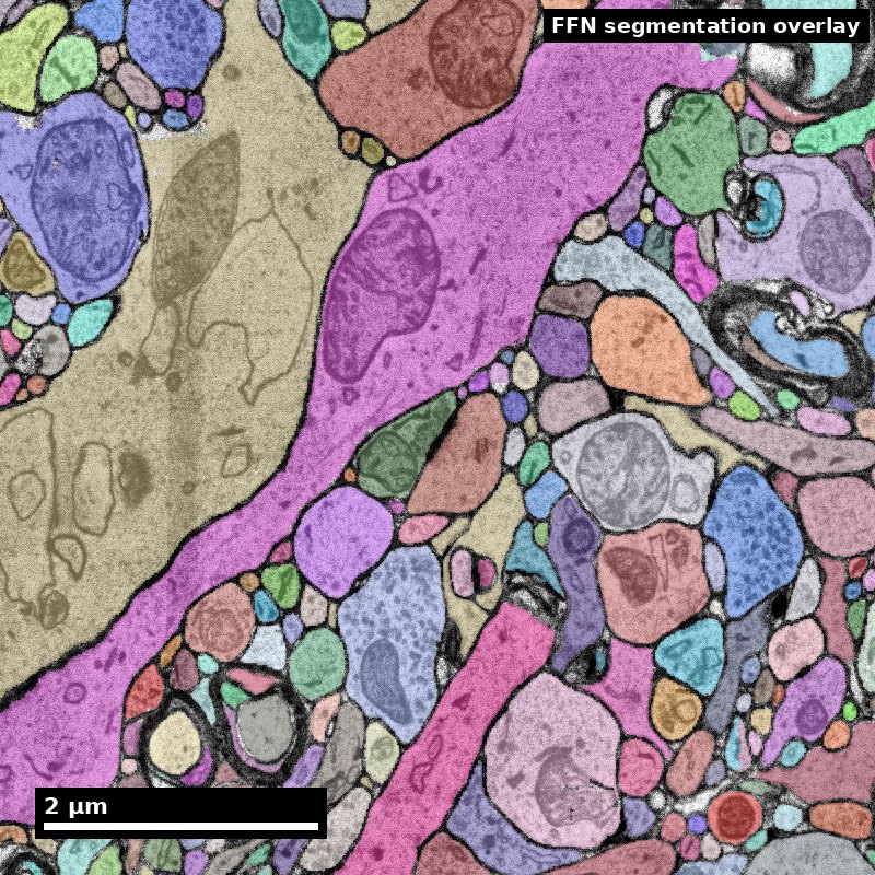
Human cortex · H01
Object segmentation over electron microscopy
H01 release · Lichtman Lab / Harvard & Connectomics at Google
Image: CC BY 4.0 · Shapson-Coe et al. (2024) · doi:10.1126/science.adk4858
Lecture: CC BY-SA 4.0 · neurotrailblazers.org
Figure description and teaching notes
Welcome. This is the first of three connectomics modules. My goal for today is not
that you leave able to run a pipeline — that is Modules 8 and 9. It is that you leave
able to read a connectomics claim and say precisely what evidence would support it.
Housekeeping before Part A: the module assignment and the journal club paper are both
on the last two slides. Journal club presenter for Module 8 should choose by end of week.
Slide 2 of 59
Where this module sits
Three modules, one argument: measure it, build it, use it
| Module | Question it answers | What you produce |
|---|---|---|
| 7 — Introduction | What is a connectome, at which scale, and what can it support? | A study brief with a measurable endpoint |
| 8 — Tools and methods | How does tissue become a queryable petascale dataset? | A reproducible query against a public volume |
| 9 — Algorithms and applications | How do you get from voxels to a defensible claim? | A motif analysis with a stated null model |
The through-line is the same in all three: a connectomics result is a measurement with a stated sampling, a stated error rate, and a stated non-claim. Everything else is illustration.
Figure description and teaching notes
Say this explicitly: the three modules are one argument, not three topics. Students
routinely treat Module 7 as "background" and skip to the tools. The claim-sorting
framework in Part A is what Module 9's lab is graded against, so it is load-bearing.
Slide 3 of 59
The discovery pipeline
One path from question to claim. Every technique in these three modules sits on it.
   QUESTION        SPECIMEN         IMAGE           RECONSTRUCTION      GRAPH        CLAIM
      |               |               |                   |              |            |
  measurable      fixation        alignment          segmentation    node/edge      null
   endpoint       staining        ingest             proofreading    definition     model
   null model     sectioning      storage            synapses        inclusion      error band
   non-claim      imaging         serving            versioning      boundary       non-claim
      |               |               |                   |              |            |
  -- Module 7 --  -------- Module 8 --------   ----------- Module 9 -----------
Read it in both directions. Left to right, it is how a dataset gets built. Right to left, it is how you debug a number you do not believe — and that is the direction you will use more often.
Every stage adds a decision that changes the answer, and every stage has a characteristic failure. The three modules walk the pipeline once, in order.
Slide 4 of 59
Learning objectives
By the end of Module 7 you will be able to:
7.1 — Explain the scope of connectomics across macro-, meso-, and nanoscale.
7.2 — Differentiate the three scales by resolution, volume, and the claims each can support.
7.3 — Classify a connectivity claim as supported by structure alone, supported by structure plus a declared assumption, or not supportable by structure.
7.4 — Communicate the current challenges and opportunities in connectomics to a technical audience without overclaiming.
Objective 7.3 is the one this module is really about, and it is the one most often failed — by students and by published papers.
Figure description and teaching notes
Note for the instructional record: these MLOs are single-verb, matching the design
guidance in the CDM review. 7.3 was split out of the old 7.2 because "differentiate
and evaluate" was double-barrelled.
Slide 5 of 59
Roadmap
Three parts, roughly fifty minutes each
Part A — The case for mapping Why electron microscopy, why it costs what it costs, and the three bins every connectivity claim falls into.
Part B — Three scales Macro, meso, nano. The modality chart, the tradeoff triangle, and how the scales are joined — and mis-joined.
Part C — The field as it stands Landmark datasets from 1986 to 2025, what each one actually delivered, and the open problems worth your attention.
Bring to each part: a brain question you actually care about. You will rewrite it three times.
Slide 6 of 59
Part A
The case for mapping
- The resolution argument, in numbers
- The cost argument, in numbers you can compute
- What structure can and cannot establish
Slide 7 of 59
A connectome, defined
A map of the connections in a nervous system, at a stated resolution, from a stated sample
What it is. A graph whose nodes are neurons (or cell types, or compartments) and whose edges are measured connections, derived from imaging a physical specimen.
What it is not:
- Not a set of synaptic weights — synapse count is a proxy for strength, not a weight.
- Not a set of dynamics — it is one animal, at one moment, fixed.
- Not a runnable brain — the map constrains the space of possible dynamics; it does not simulate them.
- Not one thing — "connectome" names three different measurements at three scales that are routinely conflated. That conflation is Part B.
Figure description and teaching notes
Push on "at a stated resolution, from a stated sample." Both qualifiers get dropped in
abstracts and both are where the errors live. Ask the room: what is the sample in the
H01 dataset? Answer: surgically resected human temporal cortex from an epilepsy
patient — which is a provenance fact with real interpretive consequences.
Slide 8 of 59
Why map: the question types only structure can answer
The "why" of connectomics, stated as a list rather than an enthusiasm
| Question type | Example | Why structure is required |
|---|---|---|
| Census | "How many cell types are there, and what does each connect to?" | Requires seeing every partner, including ones nobody labeled |
| Specificity | "Does type A target proximal dendrites of B and distal of C?" | Compartment targeting is invisible without synapse-resolution geometry |
| Comparison | "How does this circuit differ across development, sex, or species?" | Needs the same measurement twice, at the same resolution |
| Stereotypy | "How much of wiring is specified rather than idiosyncratic?" | Requires matching two complete graphs |
| Model constraint | "Which dynamical models are consistent with this anatomy?" | Removes free parameters that no functional recording can pin down |
Notice what is absent. No row says "reveals how the brain computes." Every row is a measurement whose result could come out otherwise — and each maps to a real published result you will meet in Part C.
Slide 9 of 59
Vocabulary that will recur for three modules
Neurite — any neuronal process, before you have decided whether it is an axon or a dendrite. The honest word when the call is not yet made.
Neuropil — the dense tangle of neurites and glia between cell bodies. Where essentially all synapses live, and where segmentation is hard.
Soma — the cell body. Easy to segment, and only a tiny fraction of a neuron's volume.
Supervoxel — a small over-segmented image fragment; the immutable atom that reconstructions are built from. (Module 8.)
Proofreading — human correction of automated segmentation. The dominant cost of every large connectome.
Split / merge — the two error types. A split leaves one neuron in pieces; a merge fuses two neurons into one. They are not equally bad, and that asymmetry shapes the whole field.
Materialization — a frozen, versioned snapshot of a continuously-edited reconstruction. The thing your analysis must cite. (Module 8.)
If you take one word from this slide, take merge. Module 9 spends most of Part B on why merges bias results in a specific and predictable direction.
Slide 10 of 59
Three claims about the same circuit.
Which one does a wiring diagram support?
- "Neuron X makes 42 synapses onto neuron Y."
- "Neuron X strongly excites neuron Y."
- "This circuit computes heading direction during navigation."
Hold your answer. We come back to this in eleven slides.
Figure description and teaching notes
Cold open. Do not resolve it now. Take a show of hands on each: most rooms accept 1,
split on 2, and about a third will accept 3 because it sounds like something they have
read — which is exactly the point, because they have read it.
Answers, for your own reference: 1 is Bin A, 2 is Bin B (assumes morphology predicts
sign and count predicts strength), 3 is Bin C (needs physiology).
Slide 11 of 59
The resolution argument
Connectomics exists because of a physical mismatch
| Structure | Approximate size | Resolvable by light microscopy (~200–250 nm)? |
|---|---|---|
| Cortical neuron soma | 10–25 µm | Yes, easily |
| Dendritic shaft | 0.5–3 µm | Yes |
| Myelinated axon | 0.5–2 µm | Usually |
| Dendritic spine head | 300–800 nm | Marginally |
| Unmyelinated axon in neuropil | 80–300 nm | No |
| Dendritic spine neck | 50–200 nm | No |
| Synaptic cleft | ~20 nm | No |
| Postsynaptic density | 30–50 nm thick | No |
Electron microscopy at 4 × 4 × 40 nm resolves every row. That is the entire reason the field tolerates the cost on the next slides.
Slide 12 of 59
Overlap is not connection
The consequence is specific, not general
Light microscopy can tell you that two neurons' arbors occupy the same space. It cannot tell you they are connected, because at 250 nm two membranes 20 nm apart are one blur.
In dense cortical neuropil a 1 µm³ box contains on the order of a dozen distinct neurites. Below the diffraction limit they are indistinguishable.
Peters' rule and its limits. Predicting connectivity from arbor overlap is a standing hypothesis, not a measurement. Neurons that touch frequently often do not connect, and connection probability varies strongly by cell type. Contact is a proxy whose relationship to connectivity is itself an open research question.
A colleague proposes confocal imaging of sparsely labeled neurons to "map the connectome" of a cortical column. Strongest single objection?
Figure description and teaching notes
Expected answer: sparse labeling plus diffraction-limited optics gives potential
contact, not synaptic connection. Secondary objection worth drawing out if nobody
raises it: sparse labeling means you cannot see the unlabeled partner, so even a true
synapse has an anonymous other side.
Slide 13 of 59
What EM buys, and what it does not
Resolving a synapse is not the same as knowing what it does
EM gives you an anatomical synapse:
- a presynaptic vesicle pool
- a synaptic cleft
- a postsynaptic specialization
That is a real, direct, physical observation. It is the strongest evidence the field has.
EM does not give you:
- sign — inferred from morphology (Gray type I vs II) or a separate molecular measurement
- strength — synapse count and PSD area are proxies
- state — potentiated or depressed is invisible
- neuromodulation — volume transmission leaves little trace
Every one of the four items on the right is a place where an assumption enters. Part A ends by making you name them out loud.
Slide 14 of 59
Calling a synapse: the three criteria
What "we observed a synapse" actually means, operationally
An anatomical synapse is called on converging independent evidence, not on one cue:
- A presynaptic vesicle cluster — a pool of ~40 nm vesicles gathered at the membrane, not scattered through the cytoplasm.
- A synaptic cleft — a consistent ~20 nm gap with visible density in it, held parallel over the apposition.
- A postsynaptic specialization — a thickened, electron-dense band on the receiving side (the postsynaptic density).
The classic false positive: the adherens junction. Two membranes held parallel with symmetric density on both sides and no vesicle pool. It looks like a synapse to a detector trained on apposition alone. The vesicle criterion is what excludes it.
Gray type I vs type II. Asymmetric, prominent PSD, round vesicles → putatively excitatory. Symmetric, thin PSD, often flattened vesicles → putatively inhibitory. Note the word "putatively": this is the Bin B assumption from three slides ahead, and it is the single most common unstated assumption in the literature.
Slide 15 of 59
The cost argument
Arithmetic you should be able to do in your head
Raw voxel count = volume ÷ voxel volume. Take 1 mm³ of cortex at 4 × 4 × 40 nm:
x: 1 mm / 4 nm   = 1,000,000 nm / 4 nm  = 250,000 voxels
y: 1 mm / 4 nm   =                        250,000 voxels
z: 1 mm / 40 nm  = 1,000,000 nm / 40 nm =  25,000 voxels

total = 250,000 x 250,000 x 25,000      = 1.56 x 10^15 voxels
At 8-bit grayscale: ~1.56 petabytes of raw image data for one cubic millimeter — before alignment, before segmentation, before meshes, before any derived product.
Published petascale volumes land here. H01 (human temporal cortex) and MICrONS (mouse visual cortex) are both roughly 1 mm³ and both are reported in the 1.4–2 PB range, depending on what is counted and how it is compressed.
Figure description and teaching notes
Make them do this one. It is the fastest sanity check on any proposal they will ever
review, and it takes thirty seconds. If a proposal's storage line item is off by two
orders of magnitude from this arithmetic, nothing else in it is trustworthy.
Slide 16 of 59
Now extrapolate, and notice where it breaks
| Target | Volume | Raw data at 4 × 4 × 40 nm | Status |
|---|---|---|---|
| C. elegans nervous system | ~0.00005 mm³ | ~0.1 TB | Done, repeatedly, since 1986 |
| Adult Drosophila brain | ~0.02–0.03 mm³ | ~40 TB | Done — FAFB, hemibrain, FlyWire |
| Mouse cortical column / 1 mm³ | 1 mm³ | ~1.6 PB | Done — MICrONS, H01 |
| Whole mouse brain | ~500 mm³ | ~800 PB | The current grand challenge |
| Whole human brain | ~1.2 × 10⁶ mm³ | ~10²¹ bytes | Not a plan; a horizon |
The jump that matters. Fly → mouse mm³ is ~40×. mm³ → whole mouse brain is ~500×, and it is not a jump in microscopy. It is a jump in sectioning reliability, storage economics, alignment robustness, segmentation accuracy, and above all proofreading labor.
NIH BRAIN CONNECTS (first awards 2023) exists because that 500× is an engineering program, not a microscope purchase.
Slide 17 of 59
Check yourself
You are offered beam time for 0.05 mm³ of mouse hippocampus at isotropic 8 nm (FIB-SEM). How much data, and what changes?
The arithmetic
voxel volume = 8 x 8 x 8 = 512 nm^3
0.05 mm^3    = 5 x 10^16 nm^3

5e16 / 512   = ~1 x 10^14 voxels
             = ~100 TB
What actually changed: isotropy.
At 4 × 4 × 40 nm the z-axis is 10× coarser than xy. Processes running in-plane are easy; processes crossing z steeply are hard.
That anisotropy is the single largest driver of automated segmentation error — we return to it in Module 9.
Isotropic 8 nm removes the asymmetry, at the cost of throughput and a hard ceiling on volume per run.
Slide 18 of 59
What structure can and cannot establish
Sort every claim you plan to make into one of three bins
Bin A — structure alone suffices Direct anatomical observation, or a structural statistic against a stated null.
Bin B — structure plus one declared assumption Defensible, but the assumption must be named in the same sentence.
Bin C — structure cannot establish this Requires physiology, perturbation, or molecular measurement.
The most common failure in connectomics writing:
a Bin C sentence in the abstract, supported by a Bin A measurement in the results.
This is the framework Module 9's lab is graded against. Learn it now.
Slide 19 of 59
Bin A — structure alone is sufficient evidence
-
"Neuron X makes 42 synapses onto neuron Y." Direct anatomical observation.
-
"Cell type A targets the proximal dendrites of type B, while type C targets distal dendrites." Compartment targeting is measured, not inferred.
-
"Reciprocal pairs occur 4× more often than expected under a degree-preserving null model." A structural statistic — against a stated null. Drop the null and it leaves Bin A.
-
"This projection does not exist in this volume." A negative result — with a stated detection sensitivity. Drop the sensitivity and it is not a claim at all.
Two of these four depend on a qualifier that is routinely omitted. A Bin A claim without its null or its sensitivity is not a weaker Bin A claim; it is unfalsifiable.
Slide 20 of 59
Bin B — structure plus one declared assumption
| Claim | The assumption it requires |
|---|---|
| "This synapse is excitatory." | Asymmetric (Gray type I) morphology predicts glutamatergic transmission. Usually good in cortex; still an assumption, with known exceptions. |
| "This is a strong connection." | Synapse count or total PSD area is monotonic in physiological strength. Defensible, supported in some systems — but a model. |
| "This circuit performs coincidence detection." | A biophysical model linking morphology and connectivity to integration. |
The rule. Any Bin B claim names its assumption in the same sentence, or in the figure caption. "Putatively excitatory (asymmetric morphology)" costs four words.
Slide 21 of 59
Bin C — structure cannot establish this
- "This circuit computes X during behavior Y." → requires physiology
- "This synapse is potentiated." → requires a functional or molecular measure
- "This wiring causes the animal's decision." → requires perturbation
- "Neuromodulatory state Z reconfigures this circuit." → volume transmission is largely invisible in a standard EM volume
A wiring diagram is a constraint on the space of possible dynamics, not a simulation.
This is not a counsel of despair. Bin C claims are answerable — with a second measurement. MICrONS exists precisely because someone decided to co-register two-photon physiology with the EM volume. The move is to add the measurement, not to soften the verb.
Figure description and teaching notes
That last line is the constructive turn and it matters pedagogically. Students hear
Bin C as "connectomics can't do anything interesting." The right reading is that Bin C
tells you exactly which additional experiment your question needs — which is a research
plan, not a limitation.
Slide 22 of 59
Back to the cold open.
- "Neuron X makes 42 synapses onto Y."
- "Neuron X strongly excites Y."
- "This circuit computes heading direction."
Bin A — direct observation. Bin B — assumes morphology → sign, count → strength. Bin C — needs physiology.
Claim 3 is true of the fly central complex. It took the connectome plus a decade of physiology. The connectome alone could not have established it — and did not.
Slide 23 of 59
Worked example: repairing a research question
Version 0 — "We will use connectomics to understand how the cortex implements predictive coding."
Bin C, no measurable endpoint, no result could falsify it. Four moves to repair it:
1 — Find the structural signature. Predictive-coding architectures require asymmetry between feedforward and feedback pathways. Candidate signature: feedback axons from higher visual areas target a different dendritic compartment of L2/3 pyramidal cells than feedforward L4 inputs do.
2 — Define the measurement, with units. Per proofread L2/3 pyramidal cell, the fraction of input synapses by presynaptic source class, binned by path distance from soma (0–50, 50–150, 150–300, >300 µm) and by compartment (spine head, neck, shaft, soma, AIS).
Figure description and teaching notes
Move 1 is the hard one and it is where a student's domain knowledge earns its keep.
There is no algorithm for it: you have to know the theory well enough to know what it
predicts about anatomy. This is why the module assignment asks them to do it in their
own subfield rather than in vision.
Slide 24 of 59
Worked example, continued
3 — State the null. Sources are distributed across compartments in proportion to available postsynaptic surface area.
This null is doing real work. Dendrites have more distal surface than proximal, so "more distal synapses" is the expected result and is evidence of nothing.
4 — Write the non-claim. "These data constrain where feedback input arrives on the dendritic tree. They do not establish that these synapses carry prediction-error signals, and they do not establish sign."
Version 1 (usable). "In mouse visual cortex, do inter-areal feedback axons target a systematically more distal dendritic compartment of L2/3 pyramidal cells than L4 feedforward axons do, relative to a surface-area-proportional null, measured across ≥50 proofread cells?"
Version 1 can be answered, can be wrong, and can be scoped in a grant.
Slide 25 of 59
Sizing the claim to the reconstruction
A structural claim is only as good as the completeness behind it
| Claim type | Minimum reconstruction state | Typical failure if you skip this |
|---|---|---|
| "Cell X synapses onto cell Y" | Both partners proofread through the synapse; synapse manually verified | A merge error invents the connection |
| "Cell X has n inputs" | Full dendritic arbor proofread and closed | Split errors truncate the arbor; n undercounts by an unknown amount |
| "Type A prefers type B over type C" | Both target populations proofread to comparable completeness | Differential completeness masquerades as biological preference |
| "Motif M is enriched" | A closed subgraph with quantified edge precision/recall | False edges from merges inflate dense motifs superlinearly |
| "This projection is absent" | Stated detection sensitivity and searched volume | Absence of evidence reported as evidence of absence |
Row 4 returns in Module 9. Merge errors do not add noise symmetrically. One merge fuses two neurons' partner lists, manufacturing triangles and reciprocal pairs far above the error rate itself. Motif analysis on unproofread segmentation is not conservative — it is biased toward the interesting answer.
Slide 26 of 59
Part A checkpoint — four things to stop believing
"Higher resolution is always better." No. The rule is the coarsest scale whose reconstruction resolves your analysis unit.
"If two neurons touch, they probably connect." Contact predicts connectivity poorly, and non-uniformly by cell type.
"The connectome tells you the circuit's function." It constrains the space of possible dynamics. Function needs a second measurement.
"Segmentation errors just add noise." Merges bias results toward dense motifs — the direction of the interesting answer.
Break. When we come back: why "connectome" names three different measurements.
Slide 27 of 59
Part B
Three scales that are not the same thing
- Acquisition, reconstruction, and analysis scale
- The modality chart and the tradeoff triangle
- Representations, and cross-scale linkage
Slide 28 of 59
Three scales practitioners routinely conflate
Separating them prevents most downstream confusion
Acquisition scale — the voxel size and field of view your instrument produces. Set by physics and budget. Fixed once the data exists.
Reconstruction scale — the smallest object you can reliably segment. Always coarser than acquisition scale, sometimes much coarser. At 4 × 4 × 40 nm you acquire enough signal to see a 20 nm cleft, but you can reliably segment neurites down to roughly 50–100 nm — and reliability drops sharply for processes running steeply through z.
Analysis scale — the unit your conclusions are about: a synapse, a cell, a cell type, a layer, an area, a projection.
The decision rule. Choose the coarsest acquisition scale whose reconstruction scale still resolves every object your analysis scale depends on. Not the finest you can afford — the coarsest that works.
Slide 29 of 59
The decision rule, applied
Endpoint: "fraction of inputs onto spines vs shafts"
Analysis scale = the synapse and the spine neck. Spine necks are 50–200 nm. → Reconstruction scale must be ≤ 50 nm. → This forces EM.
Endpoint: "does area A project to area B at all"
Analysis scale = the axon bundle. → Light-sheet imaging of a bulk tracer at 1 µm is not merely adequate — → it is the correct choice, because it costs about five orders of magnitude less.
Every step finer multiplies data volume, alignment difficulty, and proofreading hours. Choosing EM when light microscopy answers the question is not caution. It is a five-order-of-magnitude error.
Figure description and teaching notes
This slide is where students who came in assuming "nanoscale is the serious scale"
should be dislodged. The correct instinct is scale-matching, not scale-maximizing.
Slide 30 of 59
The modality chart
| Modality | Resolution (typical) | Practical volume | Uniquely gives you | Cannot do |
|---|---|---|---|---|
| Diffusion MRI tractography | 0.5–2 mm | Whole human brain, in vivo | Whole-brain, living, repeatable, human | No individual axons; false and missing tracts; no synapses; no direction |
| Light-sheet / whole-brain LM with tracers | 0.5–2 µm (xy) | Whole mouse brain | Long-range projection maps, many animals | Cannot resolve neurites in neuropil; no synapses |
| Confocal / two-photon | 200–300 nm lateral | mm³, in vivo possible | Function (calcium), molecular labels, live | Diffraction-limited; overlap ≠ connection |
| Expansion microscopy | ~25–70 nm effective | Up to ~mm³ with effort | Molecular identity plus near-EM geometry | Expansion distortion; not yet routine for dense reconstruction at scale |
| Array tomography | ~50–100 nm lateral, 70 nm sections | ~10⁵ µm³ | Multiplexed protein labeling at synapse-scale geometry | Section loss; lower z-resolution than EM |
| Barcoded projection mapping (MAPseq/BARseq) | Single-cell identity, no geometry | Whole brain, 10⁴–10⁶ cells | Projection patterns of enormous numbers of cells, cheaply | No synapses, no morphology, no local circuit |
| ssTEM / ssSEM (multibeam) | 4 × 4 × 40 nm | Up to ~1 mm³ today | Dense synapse-resolution reconstruction at scale | Anisotropic; section artifacts; enormous cost |
| SBEM | 10–20 × 10–20 × 25–50 nm | ~10⁶–10⁷ µm³ | Automated block-face series, no section handling | Destructive; z-resolution limits thin-process tracing |
| FIB-SEM | 4–8 nm isotropic | ~10⁵–10⁶ µm³ (more with hot-knife) | Isotropic — best tracing conditions available | Slow; limited volume per run |
Ranges are typical rather than record-setting. Learn the shape of this table, not the digits.
Slide 31 of 59
The tradeoff triangle
Resolution, volume, throughput — you may choose two
FIB-SEM buys resolution, gives up volume.
Light-sheet buys volume and throughput, gives up resolution.
Multibeam ssSEM is the current attempt to buy resolution and volume by throwing an unreasonable amount of throughput engineering at the problem — 61 or 91 beams in parallel.
That engineering is why 1 mm³ became feasible.
Read the triangle backwards. When a paper reports an impressive number on one corner, ask which corner paid for it. There is always one. If the methods do not say, that is itself the finding.
Emerging routes are attempts to change the triangle rather than to trade within it — SmartEM (ML-guided acquisition, 2025), FAST-EM array tomography (2024), and LICONN (2025), which reaches dense synapse-level reconstruction by light microscopy.
Slide 32 of 59
Different tools for different jobs
Two scales we will not cover — and why naming them still matters
Diffusion MRI tractography (0.5–2 mm) is the only method that measures a living human brain, repeatedly, in cohorts of thousands. That is a capability no other method on the chart has.
It also cannot see an axon. Every edge is a model output — streamlines inferred from water-diffusion orientation, with well-documented false continuations at crossing fibers.
X-ray microtomography (~0.1–1 µm) images large volumes non-destructively, which makes it excellent for targeting: find the region worth sectioning before you destroy the block.
It does not resolve synapses.
The transferable point, and the only one this course needs.
These are not weaker connectomics. They are instruments for different questions, with sampling that does not nest inside ours.
"Which regions are connected in this living patient?" → dMRI. "Where in this block should I spend a year of EM?" → XRM. "Does cell A synapse onto cell B?" → only volume EM.
Where it goes wrong is at the joins. A dMRI "connection" cited as a projection, then as a synapse, is the scale-leakage failure on the next slide — and it is far more common than any error inside a single method.
Slide 33 of 59
Mesoscale: projections without synapses
Tracer injection + light-sheet. Anterograde and retrograde tracers, cleared whole brains, registered to a common atlas. The Allen Mouse Brain Connectivity Atlas is the canonical product: a region-by-region projection matrix across hundreds of animals.
What it gives: long-range architecture, across many animals, with statistical power over individuals.
What it cannot give: which cell connects to which, and no synapses at all.
Barcoded projection mapping. MAPseq / BARseq tag individual neurons with unique RNA barcodes, then sequence target regions to read out where each cell projects.
What it gives: single-cell projection patterns for 10⁴–10⁶ cells — statistical power over cells, which EM cannot approach.
What it cannot give: geometry, synapses, local circuitry. Vulnerable to fibers-of-passage and barcode sharing.
Worked choice. "Do individual L2/3 cells projecting to AL also project to PM, across thousands of cells?" → barcoding. EM is wrong twice over: a 1 mm³ volume does not contain AL, PM, and the V1 somata; and proofreading thousands of complete long-range axons is not tractable today.
Slide 34 of 59
Nanoscale: the volume EM family
The only scale that observes synapses directly
Serial-section (ssTEM / ssSEM). Cut 30–50 nm sections onto grids, tape (ATUM), or GridTape; image them, often on many microscopes in parallel. The block survives imaging — so sections can be re-imaged and acquisition parallelizes. This is how petascale volumes get acquired in finite time.
Block-face (SBEM). Image the block face, shave a slice inside the chamber, repeat. No section handling, so no lost sections and far better z-alignment. Destructive.
FIB-SEM. An ion beam mills a few nanometers at a time — isotropic voxels, the best tracing conditions available. Slow, and volume-limited per run.
Choose by failure mode, not by resolution.
Serial section → lost sections, folds, chatter. Recoverable by re-imaging; costs alignment work.
Block-face → no section loss, but nothing can ever be re-imaged.
FIB-SEM → isotropy removes the dominant segmentation error, and caps your volume.
Module 8 spends Part A on exactly these tradeoffs and their artifact signatures.
Slide 35 of 59
Scale leakage
A claim measured at one scale, asserted at another, with the sampling silently dropped.
How it reads:
"Region A connects to region B" (macroscale, model-inferred) → cited as "A projects to B" (mesoscale, cell-level) → cited as "A synapses onto B" (nanoscale, never measured)
How to stop it:
Every time a claim crosses a scale, ask what new measurement licensed the crossing. If the answer is "a citation", the claim did not cross — it leaked.
This is the single most useful idea in Part B, and it costs nothing to apply. Registration residuals (four slides on) are the quantitative version of the same discipline.
Slide 36 of 59
Representations: what each one throws away
The same neuron exists in four representations, and conversions are lossy and one-way
| Representation | Size per neuron | Native operation | Discards |
|---|---|---|---|
| Volume (labeled voxels) | GB | "Is this a merge error?" | Nothing — but unusable at scale for most analysis |
| Mesh (surface) | 10–100 MB | Spine shape, surface area, apposition | Interior; voxel-level evidence |
| Skeleton (centerline) | 0.1–5 MB | Path distance from soma; morphometry | Spine geometry, calibre, surface |
| Graph (nodes + edges) | KB | Connectivity, motifs, network statistics | All geometry |
How this goes wrong. A team exports a graph, runs motif analysis, finds an enrichment. A reviewer asks whether spatial proximity explains it. The graph has no geometry, so the question cannot be answered without re-running from skeletons. Archiving skeletons costs a few GB and prevents this entirely.
Slide 37 of 59
Which representation for which question
- "How many synapses between A and B?" → graph
- "Where on the dendrite do they land?" → skeleton + synapse coordinates
- "Are spines here larger than there?" → mesh
- "Is this a merge error?" → volume, always. Every proofreading decision ultimately returns to the voxels.
The rule that saves projects. Decide which representation your endpoint requires before the pipeline runs — and keep the next-richer one archived.
Skeletons discard spine necks. Asymmetric synapses land mostly on spines, symmetric ones mostly on shafts — so the loss falls differentially on the two classes you are comparing. Archive the meshes, measure the offset on 20 cells, and either correct or report the bound.
Transferable principle: choose the representation whose native operation is your endpoint metric; reject coarser candidates by naming the discarded quantity that disqualifies them; archive the next-richer one specifically to bound the bias.
Slide 38 of 59
Cross-scale linkage: registration and its residuals
Where confident-looking errors are manufactured
-
Choose anchors. Vasculature is the best EM↔LM anchor in cortex: sparse, high-contrast in both modalities, distributed, biologically stable. Somata are second. Layer boundaries are weak — gradual and observer-dependent.
-
Fit the lowest-complexity transform that works. Rigid → affine → non-linear, in that order. A sufficiently flexible warp will align anything, including things that do not correspond.
-
Report residuals locally. A 3 µm mean over the whole volume can hide a 40 µm error in one corner. Report a residual map, or per-region distributions with the maximum.
-
Hold out anchors. Fit on a subset, measure on anchors the fit never saw. A model evaluated on its training points reports its flexibility, not its accuracy.
-
Propagate the uncertainty. 5 µm residual, somata 15 µm across and sometimes 10 µm apart → some assignments are wrong. Quantify how many; carry that number into the result.
Slide 39 of 59
Check yourself, and one standing warning
Your EM↔two-photon registration reports mean residual 2.1 µm, max 31 µm. Assign functional traces to cells?
Not globally, and not yet.
- Map residuals spatially — 31 µm is almost never uniform noise; it is a region where the transform extrapolates.
- Exclude that region, or add anchors there.
- Per-cell confidence from the local residual and local soma density. Where spacing ≈ residual, mark ambiguous rather than forcing a match.
- Report cells excluded and cells ambiguous.
Anisotropy warning — this bug is common, quiet, and expensive.
On a 4 × 4 × 40 nm stack, an isotropic Gaussian kernel, an isotropic distance metric, or an isotropic morphological operation is silently wrong by a factor of 10 in z.
Check every library call for whether it takes voxel spacing. This biases every distance-based measurement you make, and nothing will warn you.
Slide 40 of 59
Part B checkpoint — the five-minute scale audit
Apply this to your own question before Part C
| Ask | If you cannot answer it |
|---|---|
| What is my analysis unit — synapse, cell, type, area, projection? | You do not yet have a question, you have a topic. |
| What reconstruction scale does that unit force? | You will over-buy resolution, or under-buy and discover it after acquisition. |
| Which modality delivers that reconstruction scale at the volume I need? | Read the modality chart again; the triangle allows two of three. |
| Which representation is my endpoint's native operation? | Your pipeline will emit a graph and you will lose the geometry you needed. |
| If I join two scales, what is my registration residual, and its maximum? | Your cross-scale assignments have an unquantified error rate. |
Five questions, five minutes, and it front-runs most of the failures the rest of this course is about. Run it on the study brief in the module assignment.
Slide 41 of 59
Part C
The field as it stands
- What has actually been delivered, 1986 to 2025
- Where to get the data
- The open problems worth your attention
Slide 42 of 59
Eight streams the field moves along
Progress is not one curve. Read any new paper by asking which stream it advances.
| Stream | What moves forward | How you measure it |
|---|---|---|
| 1 · Scale | Volume and circuit size reconstructed | µm³/mm³ imaged; neurons and synapses reconstructed |
| 2 · Throughput and automation | Acquisition and reconstruction speed; human effort | Acquisition rate; proofreading hours per mm of cable |
| 3 · Segmentation quality | Automated reconstruction accuracy | Expected run length; split/merge rates on named benchmarks |
| 4 · Modality integration | Structure joined to other measurements | EM + function (co-registered activity); EM + molecular (CLEM, expansion, barcoding) |
| 5 · Organism and lifespan coverage | Species, sexes, developmental stages, individuals | Organism/stage coverage; n individuals per species |
| 6 · Structure → function | From wiring maps to predictive models | Connectome-constrained models; validated predictions |
| 7 · Openness and community | Lab-internal data → public platforms and community proofreading | Platform releases; community participation |
| 8 · Translation and people | Human tissue, health links, workforce | Human-sample datasets; training and outreach programs |
Why this beats a single timeline. Milestone lists gravitate to the biggest consortia. Per-stream reading surfaces the work that actually unblocked the field — throughput engineering, platforms, community proofreading — and gives you eight places to contribute rather than one race to be late for.
Slide 43 of 59
Forty years in one table
| Year | Milestone | Streams |
|---|---|---|
| 1986 | Complete C. elegans hermaphrodite wiring diagram (White et al.) | 1, 5 — and the founding proof it is possible at all |
| 2004 | SBF-SEM makes automated volume EM routine (Denk & Horstmann) | 2 |
| 2011 | Wiring specificity in retina (Briggman); functional ssTEM (Bock) | 1, 4 |
| 2013 | Dense inner plexiform layer reconstruction (Helmstaedter) | 1, 2 |
| 2014 | EyeWire: citizen-science proofreading at scale (Kim et al.) | 7, 8 |
| 2015 | Saturated reconstruction of neocortex (Kasthuri); multibeam SEM | 1, 2 |
| 2017 | Flood-filling networks (Januszewski); whole-brain larval zebrafish (Hildebrand) | 3, 1 |
| 2018 | FAFB — full adult fly brain imaged (Zheng & Bock) | 1 |
| 2020 | hemibrain: largest proofread connectome + neuPrint release (Scheffer) | 1, 7 |
| 2021 | H01 human cortex; MICrONS mm³ function+structure; C. elegans development (Witvliet) | 1, 4, 5, 8 |
| 2023 | Whole-larva brain connectome with full synaptic graph (Winding) | 1, 6 |
| 2024 | FlyWire whole adult fly brain, community-proofread (Dorkenwald); connectome-constrained models predicting activity (Lappalainen) | 1, 6, 7 |
| 2024–25 | Male CNS releases; sexual dimorphism at connectome scale | 5 |
| 2025 | MICrONS flagship (functional connectomics across mouse visual cortex); songbird basal ganglia connectome; LICONN — first light-microscopy route to dense synapse-level reconstruction | 1, 4, 5 |
Stream numbers refer to the previous slide. Bold marks the stream each milestone principally advanced. Compiled from the NeuroTrailblazers connectomics evidence map; DOIs on the references slide.
Slide 44 of 59
C. elegans, and its useful negative lesson
302 neurons, complete since 1986 — and it did not immediately explain behavior
What it established. That a complete nervous system can be mapped, and that the map is stable enough to be worth having. Cook et al. (2019) added both sexes; Witvliet et al. (2021) added eight developmental stages.
Why the developmental series matters more than the adult map. A single adult connectome cannot tell you which connections are stable and which are not. Eight stages can. Comparison controls for reconstruction biases a single measurement cannot.
The lesson, stated plainly.
Having the complete wiring diagram of 302 neurons did not immediately yield an understanding of behavior. It took decades of physiology and genetics on top of the map.
Anyone promising that a connectome will explain a brain should be asked what happened with the worm.
Slide 45 of 59
Drosophila: from one brain to a community resource
FAFB (2018) — the whole adult female brain imaged by ssTEM. A substrate, not yet a connectome.
hemibrain (2020) — ~25,000 neurons of the central brain, proofread, released through neuPrint. The first large proofread connectome.
FlyWire (2024) — the whole adult brain: ~139,000 neurons, ~54.5 million synapses, proofread by a distributed community on top of FAFB.
Male CNS and optic lobes (2024–25) — the same brain in a second sex, which makes comparison possible.
What it actually delivered — new biology, not just a bigger file:
- complete cell-type censuses
- the central complex wired as a ring attractor for heading direction
- connectome-constrained models that predicted taste and behavioral responses, which were then tested experimentally
That third item is the strongest form of connectomics result available today, and Module 9 Part C is built around it.
Slide 46 of 59
Mouse and human at 1 mm³
MICrONS — ~1 mm³ of mouse visual cortex: ~200,000 cells, ~500 million synapses, with two-photon functional imaging of the same tissue.
The important thing is not the size. It is the co-registration. Structure and function in the same neurons is what lets you ask whether wiring predicts tuning.
The answer so far: "partially, with cell-type-specific rules" — exactly the kind of result only this data type can produce.
H01 — ~1 mm³ of human temporal cortex: ~57,000 cells, ~150 million synapses, from surgically resected tissue.
Demonstrated that human tissue can be prepared and reconstructed at this scale, and immediately surfaced features rare or absent in mouse — such as axons forming dozens of synapses onto a single target.
Notice what the useful results have in common. Each is a census or a comparison — not an assertion about computation. That is the shape of a defensible connectomics result today.
Slide 47 of 59
Structure → function: three results that actually landed
The strongest form of connectomics result available today
1. Retinal direction selectivity (Briggman 2011; Kim 2014). Reconstruction showed that starburst amacrine cell inhibition onto direction-selective ganglion cells is organized by space–time wiring specificity — a structural asymmetry that predicts the computation. Structure gave the mechanism; physiology confirmed it.
2. The fly central complex as a ring attractor. The connectome showed a ring of heading-tuned cells with the recurrent and inhibitory architecture a ring attractor requires. The theory pre-existed; the wiring made it a specific, testable claim about identified cells.
3. Connectome-constrained models (Lappalainen et al. 2024). Fix a network model's connectivity to the measured fly visual connectome, fit only the remaining parameters, and the model predicts neural responses that were then tested.
Read the pattern. In all three the connectome removes free parameters and turns a vague hypothesis into a falsifiable one. That — not simulation — is what a wiring diagram is for.
Slide 48 of 59
Comparative connectomics: the underrated frontier
Comparison controls for reconstruction biases that a single measurement cannot
| Dataset | Organism | Why it matters |
|---|---|---|
| C. elegans developmental series | Nematode, 8 stages | Which connections are stable across maturation |
| Ciona intestinalis larva | Tunicate | A complete chordate larval CNS |
| Platynereis larva | Annelid | Whole-animal connectomes in a distant phylum |
| Octopus vertical lobe | Cephalopod | A learning circuit that evolved independently of ours |
| Larval zebrafish whole brain | Vertebrate | Whole-brain ssEM in a vertebrate |
| Songbird basal ganglia (2025) | Zebra finch | Motor learning; a vocal-imitation circuit |
| Fly male vs female CNS | Drosophila | Sexual dimorphism at connectome scale |
If you want a thesis question that is tractable and under-occupied, it is more likely in this table than in a bigger mouse volume.
Slide 49 of 59
Where to get the data
| Platform | Holds | Good for |
|---|---|---|
| BossDB | MICrONS, H01, Kasthuri, Witvliet, zebrafish, and more | Programmatic access to raw and segmented volumes across many datasets |
| neuPrint | hemibrain, MANC, released fly connectomes | Graph queries over frozen, released connectomes — the friendliest starting point |
| FlyWire Codex / CAVE | FlyWire whole adult brain | Whole-brain fly connectivity, annotations, community proofreading |
| microns-explorer / CAVE | MICrONS | Structure plus co-registered function |
| webKnossos | MPI datasets and hosted volumes | Browser-based annotation and proofreading |
| Neuroglancer | Any precomputed volume | Viewing — the universal client |
Start here, this week. Open neuPrint, pick a fly cell type, and look at its partners. Ten minutes of clicking will teach you more about what a connectome is than this deck can.
Module 8 covers the storage formats and query APIs behind all of these, and Module 8's assignment is a reproducible query against one of them.
Slide 50 of 59
Open problems worth your attention
The 500× problem. Whole mouse brain is ~800 PB. The bottlenecks are sectioning reliability, alignment robustness, segmentation accuracy, and proofreading labor — not microscope resolution. This is what BRAIN CONNECTS is for.
Proofreading is the dominant cost. Not compute, not storage. It is a hiring, training, retention, and quality-management problem. Module 9 Part A is largely about making that labor go further.
Molecular identity. EM gives geometry, not transcriptomic type. Bridging connectomics to transcriptomics — via CLEM, expansion, or barcoding — is open and active.
Dynamics. One animal, one moment, fixed. Function must come from a second measurement, co-registered.
Individual variability. Almost every landmark dataset is n = 1. Which features are stereotyped and which are idiosyncratic is largely unmeasured — and it is the question comparative and multi-individual work exists to answer.
Alternative modalities. LICONN (2025) reached dense synapse-level reconstruction with light microscopy. If that scales, parts of the cost argument in Part A change.
Slide 51 of 59
How fast is the field actually moving?
Reconstructed volume has grown by roughly nine orders of magnitude since 1986 — from a worm's ~0.00005 mm³ to a mouse mm³ — driven by throughput engineering, not by resolution gains. Resolution has barely changed.
Automation carried it. Flood-filling networks (2018) and learned agglomeration changed the human labor per millimeter of reconstructed cable by orders of magnitude. Without that, FlyWire and MICrONS are not affordable at any budget.
Openness followed. EyeWire (2014) and FlyWire (2024) made proofreading a community activity; BossDB, neuPrint, CAVE and Neuroglancer made the data usable by people who did not collect it.
Where the curve is likely to bend. The next 500× is not a microscopy problem. It is sectioning reliability, alignment robustness, and human proofreading hours.
Watch the throughput and automation numbers in any new paper, not the volume headline. Volume is the consequence; those two are the cause.
A useful habit: when reading a new dataset paper, find the reported human hours per millimeter of cable. Many papers omit it. That omission is informative.
Slide 52 of 59
Human tissue: provenance is an interpretive fact
Not a compliance footnote
Where human samples come from. Surgical resections — most often epilepsy surgery — and postmortem brain banking. Both carry consent frameworks, and both carry biology.
H01 is tissue from a patient with epilepsy. That is not a disclaimer; it is a variable. Any claim about "the human cortex" from that sample must reckon with the clinical context, the medication history, and the resection margin.
What this means for how you write. State the provenance in the results, not the supplement. "Human temporal cortex (surgical resection, epilepsy)" is the honest noun phrase. "Human cortex" is not.
And for how you read. When a comparative claim runs mouse-versus-human, ask whether the human sample's clinical history could produce the difference. Often it cannot be excluded — and saying so is part of doing this work credibly.
Slide 53 of 59
How to read a connectomics paper
A checklist you can apply in ten minutes
- What is the sample? Species, region, n, provenance, fixation. Is n = 1?
- What resolution, and what was the reconstruction scale? Not the same number.
- What fraction is proofread, and to what standard? "Proofread" is not binary.
- How was the graph built? Synapse threshold, inclusion criteria, boundary handling. (Module 9 Part B.)
- Which materialization version? If the paper does not say, its numbers are not reproducible. (Module 8 Part C.)
- What is the null model? For any enrichment or preference claim.
- What error rates are reported, and how do they propagate to the headline number?
- Sort the abstract's central claim into Bin A, B, or C. Then check whether the results section supports that bin.
Item 8 is the one that will make you useful in a journal club immediately.
Slide 54 of 59
Part C checkpoint — what a good answer sounds like
Weak
"The connectome shows that this circuit implements predictive coding."
"We mapped the human cortex."
"Motif M is enriched (p < 0.001)."
"The data are proofread."
Defensible
"Feedback axons target more distal compartments than L4 inputs, relative to a surface-area null, across 63 proofread cells. These data do not establish that these synapses carry prediction error."
"~1 mm³ of human temporal cortex, surgical resection, epilepsy, n = 1."
"Motif M is enriched 1.4× under a degree- and distance-preserving null; the enrichment does not survive our measured merge rate."
"Exhaustive proofreading of a 20-cell sample shifted the ratio from 3.1 to 2.8."
Every right-hand phrasing is *shorter on certainty and longer on information.* That trade is the whole professional skill.
Slide 55 of 59
Discussion forum — this week
Post by Wednesday, respond to two classmates by Sunday
Prompt 1 — Bin sorting. Find one connectomics paper published in the last two years. Quote its central claim verbatim. Sort it into Bin A, B, or C, and say what evidence would be needed to move it one bin stronger. Be fair to the paper — quote the claim as written, not as you would summarize it.
Prompt 2 — Scale matching. Describe a brain question from your own area. Name the analysis scale, then the reconstruction scale it forces, then the modality. If the answer is not EM, say so — the decision rule rewards the coarsest scale that works.
Journal club (Module 8). We will read a landmark dataset paper. Presenter chooses from: FlyWire (Dorkenwald et al. 2024), MICrONS (2025), H01 (Shapson-Coe et al.), or LICONN (Tavakoli et al. 2025). Volunteer by end of this week.
Slide 56 of 59
Module 7 assignment
Five short-answer questions plus a study brief. Due before Module 8.
Short answer (5 questions). Resolution arithmetic; the extrapolation table; a Bin A/B/C sort; a modality choice with justification; a registration-residual interpretation.
Study brief (the graded artifact). One page, on a question you care about:
| Required element | What it must contain |
|---|---|
| Question | One sentence, answerable, falsifiable |
| Analysis scale | The unit your conclusion is about |
| Modality and resolution | With the decision rule applied explicitly |
| Measurable endpoint | With units and a sample size |
| Null model | Stated in words before any statistic |
| Explicit non-claim | What these data will not establish |
The non-claim is worth as much as the rest combined. It is the sentence that distinguishes a proposal from a press release.
Slide 57 of 59
What to bring to Module 8
We shift from what to how. Module 8 follows the tissue: fixation, staining, sectioning, imaging, alignment, storage, and the infrastructure that makes a petabyte queryable.
Come with:
- a browser open to neuPrint or FlyWire Codex
- the arithmetic from Part A — you will use it to size a real acquisition
- your study brief, because Module 8 asks what it would cost
The one idea to carry forward.
A connectomics result is a measurement, with a stated sampling, a stated error rate, and a stated non-claim.
Modules 8 and 9 are about earning each of those three.
Slide 58 of 59
References and sources
Landmark datasets. White et al. 1986 (C. elegans); Cook et al. 2019 (10.1038/s41586-019-1352-7); Witvliet et al. 2021 (developmental series); Briggman et al. 2011 (retina); Helmstaedter et al. 2013 (IPL); Kim et al. 2014 (10.1038/nature13240, EyeWire); Kasthuri et al. 2015 (saturated reconstruction); Hildebrand et al. 2017 (larval zebrafish); Zheng et al. 2018 (FAFB); Scheffer et al. 2020 (10.7554/eLife.57443, hemibrain); Shapson-Coe et al. (H01); Winding et al. 2023 (larval CNS); Dorkenwald et al. 2024 (FlyWire); MICrONS Consortium 2025 (10.1038/s41586-025-08790-w).
Methods and modalities. Denk & Horstmann 2004 (10.1371/journal.pbio.0020329, SBF-SEM); Knott et al. 2008 (10.1523/JNEUROSCI.3189-07.2008, FIB-SEM); Bock et al. 2011 (10.1038/nature09802, TEMCA); Eberle et al. 2015 (10.1111/jmi.12224, multibeam); Xu et al. 2017 (10.7554/eLife.25916, long-run FIB-SEM); Phelps et al. 2021 (10.1016/j.cell.2020.12.013, GridTape); Kievits et al. 2024 (10.1515/mim-2024-0005, FAST-EM); Tavakoli et al. 2025 (10.1038/s41586-025-08985-1, LICONN); SmartEM 2025 (10.1038/s41592-025-02929-3).
Analysis and modeling. Milo et al. 2002 (10.1126/science.298.5594.824, motifs); Bassett, Zurn & Gold 2018 (model taxonomy); Lappalainen et al. 2024 (10.1038/s41586-024-07939-3, connectome-constrained models); Abbott et al. 2020 (10.1016/j.cell.2020.08.010, "The Mind of a Mouse").
Course material. NeuroTrailblazers technical training Units 01, 02 and the connectomics evidence map. https://neurotrailblazers.org
Slide 59 of 59
Use, adapt, and credit
These slides are openly licensed for community use
Licence: CC BY-SA 4.0
Creative Commons Attribution-ShareAlike 4.0 International.
https://creativecommons.org/licenses/by-sa/4.0/
You may teach from these slides anywhere, including commercially; copy and redistribute them in any medium; and re-cut, shorten, translate, restyle, or merge them into your own material — and distribute the result. No permission needed.
Two conditions. Attribution — credit the original, link the licence, and say if you changed anything. ShareAlike — distribute your adapted version under this same licence, so it stays as open as what it came from.
How to credit
Gray Roncal, W. (2026). Introduction to Connectomics (EN.585.781 Frontiers in Neuroengineering, Module 7). NeuroTrailblazers. CC BY-SA 4.0. neurotrailblazers.org/teaching/lectures/
For an adaptation, prefix with "Adapted from" and note what you changed.
Editable source. The Marp markdown is in the repository — the exported PowerPoint renders each slide as an image, so the markdown is the thing to edit. https://github.com/wrgr/neurotrailblazers
Improved something? The project would like to hear about it — open an issue.
Cover image: H01 release, Lichtman Lab / Harvard & Connectomics at Google, CC BY 4.0. Shapson-Coe et al. (2024), doi:10.1126/science.adk4858. The image retains its own licence. Cited papers carry their own licences; citation is not reproduction.